Command Line Tools

bpf

Command line interface that performs power flow. It executes using commands from a Power Flow Control (PFC) file. Example usage: bpf bench.pfc. The PFC commands (.pfc) used with bpf allow for complete power flow runs including defining the network model and commands to perform various operations such as evaluating outages. The Record Formats section describes the network model records available and the Power Flow Control (PFC) section describes the PFC syntax and commands available.

In order to process a case, bpf requires a program control file and a valid set of base case data, which may be a composite of NETWORK_DATA and BRANCH_DATA formatted ASCII files or an OLD_BASE file from a previous run of bpf, and a CHANGE file.

The PFC file either contains data used for the solution, or names files containing such data. The solution data is optionally saved on the file named in the NEW_BASE command.

Types of Processing

Input files used vary with the type of IPF processing, so it is important that you have a good understanding of the purpose of each type of file. Different program functions use the files to perform specific processes. Some major processes are:

• Basic Processing (POWER FLOW)

• Merge Base /MERGE_BASE

• Network Reduction /REDUCTION

• Outage Simulation /OUTAGE_SIM

Sample PFC file setups for each of the following solution processes are given in ??.

Creating a New Base Case

The figure below depicts the initial way an IPF case is processed and how the output is saved on a NEW_BASE file, which may then become an OLD_BASE file for subsequent change studies. The contents of the print file (PFO) are defined by the P_INPUT, P_OUTPUT, and P_ANALYSIS commands. Likewise, the contents of the fiche file (PFF) are defined by the F_INPUT, F_OUTPUT, and F_ANALYSIS commands.

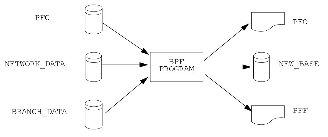
Fig. 79 New Base Creation Process

Changing an Old Base Case

The figure below shows the most commonly used bpf process. A change case is created from an OLD_BASE file using a CHANGE file. The modified case data is saved on the NEW_BASE file. The output files PFO and PFF can be printed to paper or fiche or both.

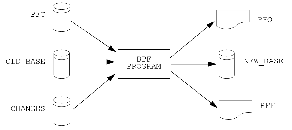
Fig. 80 Old Base Case With Changes

Merging Subsystems

The figure below shows a NEW_BASE file being created by merging a subsystem from a case on an OLD_BASE file with another subsystem from either a second OLD_BASE or from a BRANCH_DATA and a NETWORK_DATA file. The output files PFO and PFF can be printed to paper and/or fiche.

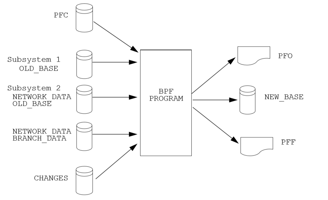
Fig. 81 Merging Two or More Subsystems

Reducing a Network

In the figure below, a network reduction is specified in the PFC file. Commands within this file define the retained system. The actual network reduction dynamically changes the base data in memory, and the reduced base case is saved on the NEW_BASE file. These output files (.PFO and .PFF) can be printed to paper and/or fiche.

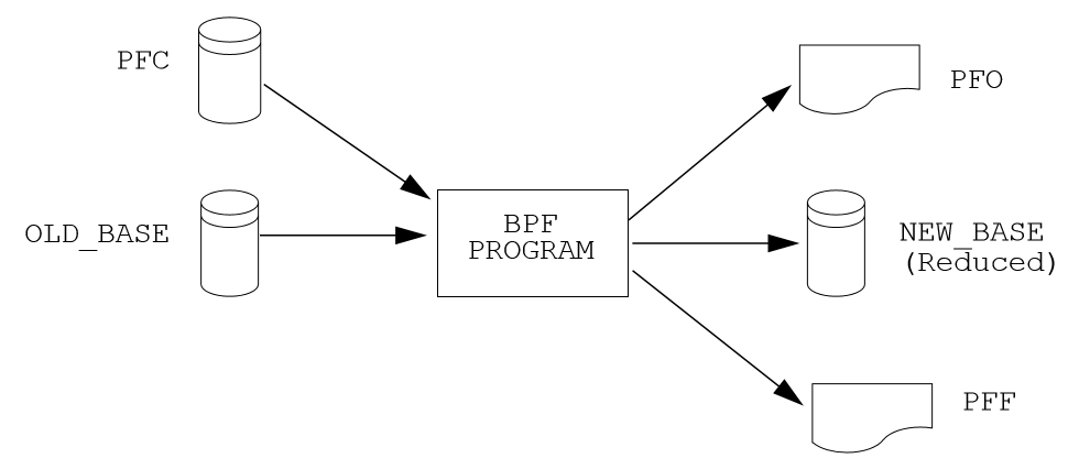
Fig. 82 Reducing a Network

For static reduction, you can use the ipfcut program. It is described in ??.

Simulating Outages

The figure below shows an outage simulation being processed directly from an OLD_BASE file. Only printed analysis is output; no data files are generated. This printed output can be directed to either fiche or paper. Simulating outages is a special power flow function that subjects a subsystem of interest to a series of single contingency branch outages and tabulates the consequences of each outage or the cause of each overload.

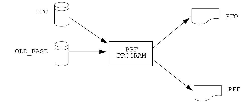
Fig. 83 An Outage Simulation

ipf_reports

ipf_reports is a command line tool that can be used to get information on an existing base case (.bse) file.

ipfplot

ipfplot is a batch plotting program to produce printed maps. The program accepts a coordinate file (.cor) and a base case file (.bse) on the command line, as well as an optional second base case file. When the second base case file is specified, a difference plot is produced. You can also use IPFPLOT to produce bubble diagrams. The same coordinate files are used for both GUI and IPFPLOT, but not all capabilities are available in the GUI.

netdat

netdat is a command line program that converts a binary base file (.bse) created by bpf to an ASCII network data file. It provides similar function to ipfnet, but ipfnet generates a network data file based on the currently loaded case in the GUI, rather than from a .bse file.

ipfcut

ipfcut is a command line program that cuts out a subsystem from a solved base case file. The full system resides in a base case file; the cut system is a card image Bus/Branch data file. Flows at the cut branches are converted into equivalent generation or load on specially formatted +A continuation bus records. An ensuing power flow run should solve with internal branch flows and bus voltages which are identical to those quantities in the original base case.

• Several methods are available to define the cut system: specifying individual buses, zones, base kVs, or individual branches.

• A pi-back feature replaces selected buses with a passive-node sequence (lines consisting of sections) with the original loads, generation, and shunts, pi-backed in proportion to the line admittances.

The function of CUTTING and REDUCTION are similar, but their methodologies are different. Both generate subsystems whose internal composition and characteristics are identical to that of the base case. REDUCTION generates equivalent branches, shunt admittances, and injections such that internal nodes still “see” the full system. CUTTING generates equivalent shunt admittances and injections such that internal nodes can determine that the boundary has changed and the external system has been cut out, even though the internal flows and nodal voltages are identical.

The CUTTING program mandates that the flow into the cut-out system is constant. This is valid for eliminating radial feeder circuits, but not for eliminating a strongly interconnected external network. In the latter case, REDUCTION yields a more responsive equivalent.

A simple criterion can be used to determine whether CUTTING or REDUCTION is more appropriate.

• Will a line outage or other major perturbation near the boundary of the retained subsystem and eliminated system significantly alter the flow between the two systems?

If the answer is no, the flow will not be significantly altered, then CUTTING is acceptable. (It is the author’s opinion that REDUCTION is always superior.)

The CUTTING program is initiated by entering ipfcut at the keyboard after the computer displays the system prompt.

From this point on the operation is interactive. You should respond to the questions as they are asked.

Cutting Methodologies

Two simple techniques are employed. Both may be used.

• Cutting the eliminated branches. In cutting, the active and reactive power flowing into a cut branch is replaced with an equivalent but fictitious load, which is appended to the terminal bus with continuation buses (+A).

• Pi-backing loads of retained buses. In pi-back, the loads and shunt susceptances on selected pi-back buses are distributed to neighboring terminal buses in proportion to their branch admittances. Only branch transfer susceptance is used (a good approximation when X >> R). Also, the pi-back bus may contain at most two branches. This corresponds with early reduction schemes. The quantities pi-backed are appended to the terminal buses on specially coded continuation cards (+A ***).

Input Commands

The syntax of CUT commands conform to the convention that has been adopted for the other IPF programs that use commands.

[FICHE, copies=n]
(CUTTING, Project=name, case ID=name)

The qualifiers that select the subsystem and enable special options are listed below:

>DEBUG<
>EXCLUDE_BUSES<
>INCLUDE_BUSES<
>PI_BACK_BUSES<
>SAVE_BUSES...<
>CUT_BRANCHES<
>SAVE_ZONES...,SAVE_BUSES...<
>WSCC<

>WSCC< Enables the WSCC option. The default is no WSCC. Special processing is effected with this option:

1. Active power flowing from a cut branch into a bus is treated as a bus load under the WSCC option. Otherwise, it is treated as a load or generation depending upon the sign of the quantity.

2. Base kV fields omit the decimal point without the WSCC option. For example, a 115.0 KV appears as “115”. Under the WSCC option, the same field appears as “115.”. The WSCC Powerflow program interprets the base fields as character instead of decimal, and those two fields are unique! Lane 115. is in New Mexico but LANE 115 is in Oregon!

3. Line sections created from pi-back are consolidated into a single equivalent pi branch with the WSCC option enabled. Otherwise, the branch records are preserved (with the necessary name changes). There is one exception: If a step-up/step-down transformer-line transformer occurs, the branch is unconditionally made into an equivalent section.

4. Any branch in the cut list that has an INT in the ownership field has its flow transferred to a +A INT continuation bus instead of a +A *** bus.

>DEBUG< Opens the program debug file. Output appears on a file with extension .pfd. This is used only by the program developers.

>SAVE_ZONES...,SAVE_BUSES...< Defines the retained network as all buses whose bases and zones both match the specified list. If SAVE_BUSES is null or omitted, only zones are considered. Continuation cards begin with a + in column 1.

For example: >SAVE_ZONES NA,NB,NC,ND,NE,NF,NG,NH, NI,NJ,NK,RM<

Any number of >SAVE_ZONE...SAVE_BASE< commands may be submitted. >SAVE_BASES...< defines the retained network as all bases whose buses match the specified list. It is not necessary to type a decimal part unless it is part of the base kV, for example, 13.8 but not 3.46. Continuation cards begin with a + in column 1.

The system is initialized as an eliminated network. The following commands define the composition of the retained system. With the exception of

>CUT_BRANCHES<, the effect of the commands may be repeated in any order. Their effects are overlaid.

>INCLUDE_BUSES< >EXCLUDE_BUSES< >SAVE_BUSES< These commands introduce buses that are specified on bus records that follow (B in column 1). >SAVE_BUSES is used to specify the entire cut system, bus by bus.

>INCLUDE_BUSES is used to expand the cut system with individually named buses. This is used in context with >SAVE_ZONES or >SAVE_BUSES to provide more flexibility in the cut system.

>EXCLUDE_BUSES is used to contract the cut system with individually named buses. This is used in context with >SAVE_ZONES or >SAVE_BUSES to provide more flexibility in the cut system.

A maximum of 1000 records are permitted. In the unlikely event that this is insufficient, the above command(s) may be simply repeated with an additional block of bus records.

>CUT_BRANCHES< This command introduces branches that are specified on line records that follow (L, T, or E in column 1). A maximum of 500 cut branch records is permitted.

The CUT_BRANCHES are oriented in the following order: retained bus, cut bus.

The cut system is defined in the following manner. Starting from the set of all cut branches, each bus on the cut side, which is in the eliminated system, is expanded one-adjacent by examining each branch connected to that bus. All branches that are not connected to any bus on the retained bus side are in the cut system. Those terminal buses are eliminated.

The first pass determines all buses 1-adjacent that are in the cut system. The process is repeated, starting with all buses 1-adjacent to the cut boundary to find all buses 2-adjacent. This process is repeated until no further expansion occurs in either system. The major advantage of this approach is that any incomplete cut enclosure is properly diagnosed near the missing branch.

If the WSCC qualifier is selected, any branch in the cut list that has an INT in the ownership field will have its flow transferred to a +A INT continuation bus instead of a +A *** bus. This is done so that if this cut system is to be reintegrated into another system the cut points can be easily identified and discarded.

Unlike other >...< commands, CUT_BRANCH cannot be repeated.

>PI_BACK_BUSES< This process replaces a bus having one or two branches with an equivalent consisting of bus generation, load, and shunt admittances on the adjacent terminal buses.

If the bus originally had two branches, the new system has the following changes:

• The buses’ generation, load, and shunt admittance are proportioned by the branch admittance to each terminal node.

• The bus is eliminated.

• The subsystem consisting of a bus and two branches is replaced with a single branch spanning the two terminal buses.

If the bus originally had one branch, the new system has the following changes:

• The buses’ generation, load, and shunt admittance are transferred to the terminal node.

• The bus and its branch are eliminated.

In essence, a pi-backed bus becomes a passive node in a branch that now consists of sections. Since the quantities are pied-back in proportion to their branch admittances, the redistribution approximates the effects of REDUCTION. A maximum of 1000 pi-back records may follow. If this limit is insufficient, the remaining pi-back records may follow another >PI_BACK< command.

Interactive Approach

The following is an example of the dialogue that occurs during an interactive execution.

* command file is: J8301FY84.CUT
ENTER NAME for BUS/BRANCH output file > J83CUT.DAT
ENTER file name for OLD_BASE > A8301FY84.BSE

pvcurve

pvcurve is a command line program that automates production of power (P) voltage (V) curve plot files and plot routine setup files for multiple base cases and outages.

post_pvcurve

post_pvcurve is a command line program that ?

qvcurve

qvcurve is a command line program that generates power-reactance curves.

findout

Command line interface that Generates a table of outages and corresponding branch overloads or bus voltage violations from power flow output (.pfo) files. Works with the .pfo output files of bpf runs that contain an /OUTAGE_SIMULATION command. Runs as a post-processor to filter and sort the results and present them in tabular form. Tables of ‘Outages and Overloads’ or ‘Outages and Bus Violations’ can be produced. Entries in these tables can be filtered according to Zone, Owner, Base kV, Loading and Bus Voltage.

Tables can be sorted by Zone, Owner, Base kV, or alphabetically. The idea is to allow the user to automate the creation of a report detailing the results of outages instead of having to do manually which generally includes cut and paste operation with a text editor. Data fields in the output report table are character delimited to ease importing to Microsoft Excel or DECwrite.

lineflow

lineflow is a command line program that generates a table of values showing the requested branch quantities for multiple base cases. Selects lines by branch list, bus, kV, owner, zone, loading level, or matches to ‘wild card’ input. Sorts alphabetically, or by owner, zone, kV, loading (in percent), or according to input order of branches in a list. Generates a control script that allows repetitive similar studies to be performed automatically. Reports the following quantities: loading in Amps or MVA and percent of critical rating; or, power in, power out, and losses in MW. Data fields in the output report table are character delimited to ease importing to Microsoft Excel or DECwrite.

mimic

mimic is a command line program that generates new cases given a list of base cases and a list of change files. Check the new cases for over and under voltages, overloads, and excessive voltage and loading changes.

ipfsrv

ipfsrv is a service daemon which acts as the power flow server backend component of the X Window Graphical Interface (gui). It executes Powerflow Command Language (PCL) commands dispatched from the gui. It gets launched automatically by the gui.

ipfbat

Overview

ipfbat is a command line program that is the batch version of ipfsrv. It accepts a Powerflow Control Language (.pcl) file. Plotting can be done with a control file; however, for most plots ipfplot is easier to use. Example of use: ipfbat bench.pcl. The PCL commands used with ipfsrv and ipfbat are described in Powerflow Command Language (PCL).

Batch Mode Plotting

Batch mode plotting can be used when a coordinate file already exists, and the user simply wants a hard copy diagram based on that file and Powerflow data. If the Powerflow data is on a saved base case (*.bse) file, the simplest method is to use the ipfplot program. However, ipfbat offers more flexibility and control. For example, with ipfbat you can load, solve, and plot a netdata file.

This technique can be used to produce diagrams that are generally produced through the GUI or for access to features that have not yet been implemented in the GUI. These features include plotting bubble diagrams, plotting difference diagrams, and plotting diagrams from a master list of coordinate files.

An example of batch mode plotting is accomplished through the ipfbat program as follows:

ipfbat bubble.pcl

where the .pcl file is a control file with the IPF commands and data necessary to produce a hard copy diagram.

Commands in the examples are record groups starting with a / (slash) command and ending with the next / (slash) command or (end) for the last command in the file.

Under the command /plot, the first line must name the coordinate file to be used, and the second must name the output PostScript file to be produced. Any subsequent records following, before the next /command, are interpreted as comments, and will be placed in the standard position following the last comment defined in the coordinate file.

Two special uses for comment records must be noted. If the record begins with an ampersand (&), it will be interpreted as an instruction to append the auxiliary coordinate file named on the record. At most one such file may be named. If the record begins with an ‘at’ symbol (@), it will be interpreted as an option record. Any diagram option indicated on this type of record will override the option specified in the coordinate file. Multiple @ records are allowed and will not be printed on the diagram.

Example 1

Make a “standard” diagram (similar to the GUI operation).:

/network_data,file=a92cy91.dat        ! Load the powerflow network data
/solution                             ! Solve the powerflow case
/plot                                 ! Make a hard copy diagram
aberdeenmetric.cor                    ! using this coordinate file
diagram.ps                            ! to build this postscript file.
Case prepared by: A. Perfect Planner  ! Include this comment
Priority of study: RWI                ! and this comment
&aberdeeninset.cor                    ! and this additional coordinate file.
@OPtion DIagram_type=Pq_flow          ! Supplement/Override *.cor options.
/syscal                               ! Hello operating system ...
lpr diagram.ps                        ! ... send this file to the printer.
/exit                                 ! This job is finished.
(end)

Example 2

Make a bubble diagram.

/old_base,file=j94cy91.bse ! Load the powerflow saved base case /plot ! Make a hard copy diagram bubble.cor ! using this coordinate file diagram.ps ! to build this postscript file. BUBBLE PLOT EXAMPLE ! Include this comment. /syscal ! Hello operating system … lpr diagram.ps ! … send this file to the printer. /exit ! This job is finished. (end)

Example 3

Make a difference diagram.:

/old_base,file=9_bus_test.bse                   ! Load the powerflow saved base case
/get_data,type=load_ref_base,file=bus_alt1.bse  ! Load a reference
                                                ! saved base case
/ get_data, type = load_ref_area                ! load reference solution data in tables
/plot                                           ! Make a hard copy diagram
9bus_metricdif.cor                              ! using this coordinate file
diagram.ps                                      ! to build this postscript file.
Case prepared by: A. Perfect Planner            ! Include this comment
Priority of study: RWI                          ! and this comment
Difference plot between two cases               ! and this comment.
/syscal                                         ! Hello operating system ...
lpr diagram.ps                                  ! ... send this file to the printer.
/exit                                           ! This job is finished.
(end)

Example 4

Make a series of diagrams from a list of coordinate files.:

/old_base,file=/shr5/j96cy89.bse       ! Load the powerflow saved base case
/plot                                  ! Make a hard copy diagram
master.cor                             ! using all the coordinate files
                                       ! listed in this file
diagram.ps                             ! to build this postscript file.
Case prepared by: A. Perfect Planner   ! Include this comment
Priority of study: RWI                 ! and this comment on each diagram.
/syscal                                ! Hello operating system ...
lpr diagram.ps                         ! ... send this file to the printer.
/exit                                  ! This job is finished.
(end)

Example 5

Here is an example of a master coordinate file (master.cor).:

master
/home/dave/cor/3rdac.cor
/home/dave/cor/500bus.cor
/home/dave/cor/bubble.cor
/home/dave/cor/sworegon.cor
/home/dave/cor/nwmont.cor

ipf_test

ipf_test is a command line program that provides an interactive way to run Powerflow Control Language commands. It is similar to ipfbat but prompts the user for input data rather than reading the power flow commands from a file.

ipfnet

ipfnet is the batch version of the “save netdata file” function built into the GUI / ipfsrv. This program generates a WSCC-formatted network data file in any of the following dialects: BPA, WSCC, or PTI. The GUI allows you to save a network data file describing the case you currently have loaded. This should not be confused with the netdat program, which performs very similar function by loading a saved base case (.bse) file and writing it out in an ASCII network (.net) file.

Both programs generate a WSCC-formatted network data file in any of the following dialects: BPA, WSCC1, or PTI. “Dialects” means that although the file is still WSCC format, the data is generated with special processing or restrictions and is destined for use with other programs. In the case of the PTI dialect, that data is intended to be processed by the PTI-proprietary conversion program wscfor.

This program extracts network data from a Powerflow “old base” history file. Table F-1 below summarizes the effects of each dialect.

Table 65 Effect of Dialects on Network Data File

Record or Field	Dialect	Effects
Header comments	PTI	Three header records: “<case_name> ” “<case_name> ” “<case_name> “
	BPA, WSCC, WSCC1	./CASE_ID = <case_name> ./CASE_DS = <case_description> ./H1 <header 1 text (auto-generated)> ./H2 <header 2 text (user input)> ./H3 <header 3 text (user input)> ./C001 <comment 1 text> … ./Cnnn <comment nnn text
Area “A” records	BPA, PTI	Encode zones 1-10 in “A” record, zones 11-20 in “A1” record, etc. Note: Voltage limits on “A” records are not encoded. They are specified by a default array that establishes limits using base kV and zones.
	WSCC, WSCC1	Encode only “A” record (any zones 11-50 will be lost). Note: Voltage limits on “A” records are not encoded.They are specified by a default array that establishes limits using base kV and zones.
Intertie “I” records	BPA, PTI	Single entry (low alpha to high alpha) associated “I” records follow each “A” record.
	WSCC, WSCC1	No “I” records encoded.
Default percentages on type BG buses	BPA	BG percentages are not changed.
	PTI, WSCC, WSCC1	BG percentages are calculated if their default value is invalid.
Continuation “+”” bus records	BPA	“+” records are encoded.
	PTI, WSCC, WSCC1	“+” records are consolidated with “B” records.
Reactive capability “Q” records	BPA	“Q” records are encoded.
	PTI, WSCC, WSCC1	“Q” records are not encoded.
Minimum branch impedance	BPA, PTI	Branch impedances are not changed.
	WSCC, WSCC1	Minimum branch impedances are set to 0.0003 p.u.
Branch ratings	BPA	Options: 1. Use extended ratings (120-character records). 2. Replace nominal rating with minimum (Emergency, Thermal, or Bottleneck). 3. Use nominal rating only.
	PTI, WSCC, WSCC1	Options: 1. Replace nominal rating with minimum (Emergency, Thermal, or Bottleneck). 2. Use nominal rating only.
Branch sections	BPA	Encode as originally submitted.
	PTI, WSCC	Encode all branch sections in a consistent orientation.
	WSCC1	Consolidate all sections into an equivalent branch
Regulating “R” records	BPA	Encode as originally submitted.
	PTI, WSCC	Encode as adjustable tap side-fixed tap side. 2. Consolidate parallel LTC transformers into a single, equivalent parallel LTC transformer.
	WSCC1	Encode as adjustable tap side-fixed tap side. 2. Consolidate parallel LTC transformers into a single, equivalent parallel LTC transformer. 3. Convert taps into steps (STEPS = TAPS - 1).
D-C “LD” record	BPA PTI, WSCC, WSCC1	Encode as originally submitted. Encode as rectifier side-inverter side.

The resultant output is an ASCII file. Two formats are available for the resulting output. The BPA format retains all of the extra features that are available in the BPA Powerflow program without making any modifications to the data, while the WSCC format option consolidates and restricts the features in order to be used with WSCC’s IPS Powerflow program.

The CASEID of the power flow case data being extracted is used to create a file named CASEID.DAT. Any changes made to the data for WSCC (IPS) compatibility will be flagged on file CASEID.MES.

Input

The ipfnet program prompts with the following requests:

• File name of the Powerflow “old base” history filename.

• Select output format desired: BPA, BPA1, BPA2, WSCC (IPS), or WSCC1 (IPS1).

Sample Run

Type ipfnet at the system prompt and press the <RETURN> key. Answer the questions appropriately. An example is given below.

$ ipfnet
> Enter OLD_BASE file name (or Q to quit): ../dat/43bus.bse
> Enter name of network file (default is "../dat/43bus.net"): new.net
> Enter dialect (BPA, WSCC, WSCC1 or PTI): WSCC
> Enter record size (80 or 120): 80
> Nominal rating replacement code
    T = Thermal  E = Emergency  B = Bottleneck
    T: Transformers = T, Lines = T
    E: Transformers = E, Lines = T
    B: Transformers = B, Lines = B
    ET: Transformers = E, Lines = T
    EB: Transformers = E, Lines = B
    M: Transformers = min(TEB), Lines = min(TB)
> Enter rating replacement code: T
* Options selected - dialect = WSCC
                       size  = 80
                      rating = T
> Are above options correct (Y or N)? Y

Note

The codes for dialect and rating must be upper case. ipfnet formats commands which are sent to ipfsrv. Some input checking is done, but invalid values may cause unexpected results.

ips2ipf

The Record Formats used by IPF are defined in ASCII format and consists of area, bus, and branch records. This format is very similar to the format used by the Western Systems Coordinating

Council (WSCC) back in the 1990s in their similarly named Interactive Powerflow System (IPS) application. However, note that IPF supports many record types which are not recognized by IPS, and in some cases the interpretation and application of the data values entered is different.

The ips2ipf command line program is designed to ease the burden of converting an IPS data deck into one which can be input to the IPF program with the expectation of getting the same powerflow solution results, within normal engineering tolerances. However, the conversion is not 100% automatic. See IPS IPF Differences section for more detail on the data input and internal modeling differences between the two programs.

Before running ips2ipf on an IPS data file, you should remove from the file all COPE commands (TITLE, NEW, ATTACH, etc.) The program will handle the standard ‘control cards’ HDG, BAS, and ZZ. Title records may be retained by putting an HDG in front of them, or by putting a period (.) in column 1 of each. An unlimited number of (.) comments are is allowed, but these only annotate the data; they are not printed anywhere in the output.

ips2ipf performs the following tasks:

1. Renames duplicate buses.

   IPS uses a 12-character bus name, which includes the base kV. IPF uses only 8 characters, plus the real value of the base kV. To IPS, SAMPLE 230. and SAMPLE 230 are two different buses; to IPF they are the same bus.

   ips2ipf identifies duplicate names and generates a different name for one of them. It reports any changed names; if you don’t like the name it generated, you can change it after the fact.

2. Makes the system swing bus a BS bus, if given its name.

3. Transfers non-zero shunt vars from BE and BQ records to +A records.

In IPS, the shunt vars value entered for a bus which has variable var output is considered to be a fixed component of the total vars. In order to retain this philosophy in IPF, it is necessary to put the shunt on a +A (continuation bus) record. Shunt vars entered on the BE or BQ record are considered by IPF to be continuously variable.

4. Converts non-zero ‘steps’ on R records to ’taps’ (by adding one).

   IPS uses the number of steps available between TCUL taps; IPF uses the number of actual taps. If you run the conversion on an already converted file, another one will be added, which is probably not desirable.

5. Converts IPS comments (C in column 1) to IPF comments (. in column 1).

   Unlike IPS, which prints the comments in the input data listing, IPF does not print them at all. But they can remain in the data file itself for information as long as they have a period in column 1 instead of a C.

6. Copies the controlled bus name from each X record to the corresponding BX record, to ensure that the proper bus is being controlled.

7. Copies the voltage limits from a BX record controlling a remote bus, to the remote bus record.

8. Corrects blank section id’s in multi-section lines.

   Blank is acceptable to IPF as a section identification only on single-section lines. ips2ipf identifies multi-section lines, and changes blank to 1, 1``to ``2 etc. If there are actually 10 sections (IPS limit), then sections 8 and 9 will be combined and labeled 9.

9. Gives bus ties a small impedance.

   IPF does not allow bus ties (0.0 impedance produces a fatal error.) ips2ipf changes this to (\(0.0 + j0.00001\)), the same impedance IPF gives you when you sectionalize a bus and create a “bus tie” between the new bus and the old one. However, you should note that this may cause difficulties in getting a solution. (There are no zero impedance lines in standard WSCC study cases.)

10. IPF has no RF model. Any RF records in your deck will be ignored.

Items which are not handled by ips2ipf, which you need to look out for, are the following:

11. In IPS, line and bridge current ratings on DC are not processed, but only passed on to the Stability program. IPF actually uses them. You may find that the bridge current rating on the Intermountain DC line is too low.

IPS IPF Differences

1. Powerflow Command Differences: All IPF commands are different from those in IPS. When you are using the GUI, you will not have to worry about any of these, but there are some things you will need to do to your input data deck, such as deleting all the IPS control records and COPE commands (HDG, BAS, TITLE, ATTACH, $DONE, END, etc.).

2. Terminology: The IPF Base Case (.bse) file is a binary file equivalent to the IPS History (.HIS) file. However, the Base Case file does not contain any mapping data, and only one case per file is permitted. The IPF Network (.net) file is an ASCII file equivalent to the IPS base case or base data file (.IPS). However, this file must not contain any modification records (’M’ or ’D’ in column 3). Changes go in a different file, which must be loaded separately. All mapping data is saved (in PostScript format) in a Coordinate file (.cor). Only buses which have a match in the currently loaded system data will be displayed.

3. Case Title: IPF builds the first line of a three-line IPS style title from the 10 character Caseid and the 20 character case description fields, and the other two lines from the two HEADER records. All of these are printed on standard BPA output listings, saved on the base case (history) file, and printed on hardcopy maps.

4. Structure: The IPF Changes file (.chg) contains new and modification records you want to apply in bulk to your base case (e.g. your own local system representation). You will use the GUI to make individual touch-up or particular study changes. The system slack bus must be specified as a ’BS’ bus in the Network file; there is no GUI provision for selecting a slack bus (other than by changing the type of some bus to BS).

5. Data Differences: IPF system data is very similar to that for IPS, but is not identical. If you try to read in a WSCC base case deck as an IPF network file, you can expect numerous data errors and no solution. If you charge ahead, fixing fatal errors as you stumble over them, you will still probably not get the answers to match, because of modeling differences. The data conversion program handles most of these. There are two categories of differences between BPA and WSCC power flow models:

1. Modeling differences (including BPA extensions).

2. Input data differences

	WSCC’s IPS	BPA’s IPF
1	The DC line current rating is used only as a base by IPS. Both line current and bridge current ratings are passed to the Stability program; they are not used as limits in the powerflow solution.	The minimum of the bridge current rating and the line current rating is used as a limit by the DC system solution
2	Type RM phase shifters (controlling :math: P_{km} between \(P_{min}\) and \(P_{max}\)) will bias the phase shift angle towards the original phase shift angle.	Type RM phase shifters (controlling \(P_km\) between \(P_min\) and \(Pmax\)) will bias the phase shift angle to zero degrees to minimize circulating real power flow. WSCC bias is available as a solution option on the GUI.
3	A type BG generator may control only bus type BC.	A type BG generator may control bus types BC, B , BQ, BV, and BT.
2	An LTC may control only bus type BT.	An LTC may control bus types BC, B , BQ, BV, and BT.
5	Only one voltage control strategy per bus.	A generator and an LTC may simultaneously control a common bus. If a degree of freedom exists, the LTC will control \(Q_km\) directly to minimize transformer var flow between terminal buses.
6	Type BX buses will bias the solution towards the original \(X_shunt\).	Type BX buses bias the solution to \(V_max\). WSCC bias is available as a solution option on the GUI.
7	Infinite default limits are assigned to type BG buses.	Default global voltage limits are assigned to all buses, including type BG buses, by base voltage level.
8	The bus shunt reactive on type BQ buses is fixed.	The bus shunt reactive on type BQ buses is continuously adjustable (0 to 100%). To make that quantity fixed, it must be entered on an accompanying +A continuation bus record. The conversion program automates this.
9	Inductance (G-jB) is applied to only one end of a transformer branch.	One half of G-jB is applied to each end of both transformers and balanced pi lines.
10	Model RF phase shifter takes several iterations to get from an initial angle to its final (fixed) phase shift angle.	No such model. Problems in solving phase shifters are handled internally.
11	Phase shifter must have same base kV at both terminals.	Step up phase shifter. Tap2 field is off-nominal tap2.
12	Phase shifter cannot be a section.	Phase shifting transformer can be a section.
13	Bus ties (zero impedance lines) receive special handling in solution and reporting.	No special bus tie model. A ‘bus tie’ is defined as a very low impedance line (0.0 + j0.00001).
14	Not available.	+ continuation bus records. Except for constant current load models, these records are used mainly for accounting purposes to differentiate generation, load, and shunt with unique ownerships.
15	Not available.	I area intertie records. These records compute net area export on accompanying A records.
16	Not available.	A area record may be accompanied with A1, A2, A3, and A4 continuation records to accept a maximum of 50 zones per area.
17	Not available.	Branch records accept extended line current ratings: For types L and E records, thermal and bottleneck ratings. For types T and TP records, thermal, bottleneck and emergency ratings.
18	Not available.	Types BM and LM multi-terminal DC data.
19	Not available.	Type RZ RANI devices.
20*	Base kV field interpreted as A4 for identification purposes. SAMPLE 20.0 and SAMPLE      20 are different buses.	Base kV field interpreted as F4.0. SAMPLE 20.0 and SAMPLE      20 are the same bus.
21*	The number of steps on R records are interpreted as steps, where STEPS = TAPS - 1	The number of steps on R records are interpreted as number of taps, where TAPS = STEPS + 1
22*	A parallel branch consisting of sections will accept section numbers in the set [0-9]. (Blank is interpreted as a zero.)	A parallel branch consisting of sections will accept section numbers in the set [1-9]. Zero or blank can be used as a section number only be used on delete, to remove all sections of one circuit.
23*	Remotely controlled bus for a BX bus is specified on the X record.	Remotely controlled bus for a BX bus is specified on the BX record.
24*	Voltage limits for a bus remotely controlled by a BX bus are specified on the BC record.	Voltage limits for any bus, no matter how it is controlled, are specified on the controlled bus record.
25	Voltage limits (for reporting over and under voltage buses) are specified on A records	Default voltage limits (for all purposes) are specified by a default array which establishes limits using base KV and zones.
26*	Branches entered with both R and X equal to zero receive special handling as ‘bus ties’.	Zero impedance is not allowed - no bus tie simulation.
27*	The system slack bus can be designated as a BS type bus, but very often is specified in the SOLVE options instead.	System slack bus must be specified as a ``BS `` bus.
28*	IPS accepts various types of comment records (CB, CL, CR) which annotate the data file, and are printed in the (batch) input listing.	IPF uses a .` (period) in column 1 to designate a comment. These annotate only the data file; they are never printed.

• The conversion program will handle this item.