This section describes the batch Power Flow Control (PFC) language and its syntax, commands and subcommands. Command entries follow the PFC description in alphabetical order. The table below helps you turn quickly to a specific command entry. The table also gives you a quick description of all of the commands.
Each command entry explains the meaning of the command and gives its syntax. Some commands have subcommands, which are also described. Many entries have additional discussion, and some have examples, particularly where a command’s usage may not be immediately obvious.
The bpf Power Flow Control language (PFC) consists of a sequence of program control statements, each of which in turn consists of commands, subcommands, keywords, and values. All statements have a reserved symbol in column 1 to identify a command or subcommand.
Every statement is scanned, and each command or subcommand found is compared with a dictionary in the program to find the relevant instructions. With the exception of the identifier in column 1 of each statement, PFC is free-form. All statements must be in the PFC file.
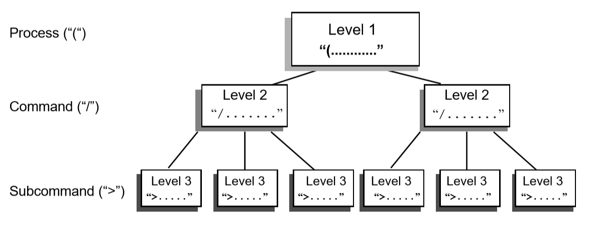
PFC has three levels of control, which are identified by one of three identifiers in column one.
The left parenthesis ( identifies the top (or process) level of control. Only four commands are valid here — (POWERFLOW, (NEXTCASE, and (STOP or (END.
The slash / identifies the second (or command) level of control. Many commands are valid here, and they are listed and described in this chapter. Commands generally enable or disable output options, define parameters needed for the process, etc. Subprocesses are major operations involving considerable processing and additional data. Only optional IPF processes are requested with these commands.
The right angle bracket > identifies the third (or subcommand) level of control. A few commands have subcommands associated with them. These subcommands are described in the associated command entries. These subcommands act as qualifiers for the second-level commands.
In addition to the foregoing syntactic units, a command enabling a microfiche option is available. Its control symbol is the left square bracket ([)
Almost every PFC statement fits one of the following formats, and the few that do not are very similar.
Note
Spaces can be used for readability. Commas are used to separate syntactic units such as a list of values or keyword/value assignments.
Most statements fit on one line, but some extend over multiple lines. These exceptions are noted. When used, put a hyphen (-) where you want to break and continue the command parameters starting in or after column 2 of the next line, column 1 must be blank.
Each general format is followed by an example.
A simple command with no keywords or values:
/command/REDUCTION
A command assigned a simple keyword. (This is a “telescoped” syntax available for some commands.)
/command=keyword/AI_CONTROL=CON
A command followed by a comma with a keyword. (This is a “telescoped” syntax available for some commands.)
/command,keyword/F_INPUTLIST,NONE
A command followed by a comma with a value assigned to a keyword.
/command,keyword=value/P_ANALYSIS_RPT,LEVEL=4
A command followed by a comma with multiple values assigned to a keyword. Note optional continuation with hyphen (-).
Two special characters are available to document the control stream or to improve readability.
A period (.) in column 1 of a record identifies a command comment and the record will be ignored by the processing. It is used to document a PFC file or to improve readability. This comment is only visible in a listing of the PFC file or in the editor used to create it.
The underscore symbol _ has no syntactic significance and may be used freely to punctuate a word for visual readability.
Note
The hyphen or minus sign “-” and the underscore “_” symbol are different characters! Thus, P_O_W_E_R_F_L_O_W is the same as POWER_FLOW which is the equivalent of POWERFLOW. OLD_BASE is the same as OLDBASE but not the same as OLD-BASE, etc.
All default values for a command are listed on the first line in the command descriptions. Various keywords are listed below the default values. Default values have been selected to satisfy a majority of users; therefore, their use is to invoke exceptions to standard conventions. Once a default value has been enabled, it remains in force for the duration of the process. There is one exception to this:
/P_INPUT_LIST
After the first case has been processed, P_INPUT_LIST is set to NONE. This conforms to the default philosophy of selecting all options that fulfill a majority of requirements.
This command requests “n” copies of microfiche listings to be made. If it is omitted, the fiche file is not saved. If “”n” is zero or omitted, no copies are made. When it is used, this control must be first in the job stream.
This command initiates the processing of the network which is defined with subsequent commands and subcommands.
(NEXTCASE)
This is the same as (POWERFLOW) except that the base network to be processed is the current network. Changes are expected; otherwise, the same network is processed again with the same data and controls in memory from the previous case. (NEXT_CASE) cannot be the first command in a program control file.
(END) or (STOP)
This stops the execution of the IPF program.
Each network is processed with a (POWERFLOW) or (NEXTCASE) command. The first must always be (POWERFLOW). Several cases may be concatenated (stacked) in the following format:
``( POWERFLOW )`` statement for case 1
``( POWERFLOW )`` statement or ``( NEXTCASE )`` statement for case 2
.
.
.
``( POWERFLOW )`` statement or ``( NEXTCASE )`` statement for case n
``( STOP )``
The following control statement and the optional keywords that go with it identify the OLD_BASE file, optionally perform miscellaneous temporary changes to OLDBASE, set solution parameters, and solve the resultant network.
(POWERFLOWCASEID=<casename>,PROJECT=<projname>)
casename is a user-assigned 10-character identification for the case. projname is a user-assigned, 20-character identification for the project or study to which this case applies. (No blanks are allowed; use hyphens instead.)
The following statement is used if the Powerflow solution is to be run starting with data and controls from the previous base case in residence.
(NEXTCASE,CASEID=<casename>,PROJECT=<projname>)
Note that /OLD_BASE is not used with a (NEXTCASE) statement since a base data file is already in residence.
Each Level 2 statement starts with a slash (/) in the first position.
After the slash are keywords and/or values separated by a comma (,). Specific values are assigned to the keywords in the following format:
keyword=value
When a keyword is requesting a list, for example, a zone list, the list may be continued on the next record by leaving column 1 of that record blank or by putting a comma in column 1 and continuing the list.
Level 3 statements consist of subcommands that specify keyword values for second-level commands only. Each subcommand for level 3 statements starts with the right angle bracket (>) in column 1. After the right angle bracket are keywords and/or values separated by commas (,). Most often, specific values are assigned by following a keyword with an equal sign (=) and then the desired value.
The rest of this chapter discusses all the PFC commands, in alphabetical order. Each command entry includes the details of syntax and usage. The more involved commands show examples of use. Refer to the table below to locate a PFC command quickly.
In the format statement for each command, the keywords and parameter values are all vertically aligned in the same column. The top row is the default value. Alternate value assignments such as ON or OFF are identified by the appropriate symbols and have the syntax keyword=value.
Required text is shown in UPPER-CASE while parameter values specified by the user are printed in lower-case and usually enclosed by angle brackets, thus, <list>. Angle brackets are omitted when they may cause confusion with the Level 3 control symbol.
The optional underscore symbol (_) may be used to break up words for visual readability. The computer will read the words as though they were not broken.
This command emulates automatic generation control (AGC) in the solution algorithm. Under AGC, real power excursions on several generators from base values are allocated in proportion to their total excursion. This in effect distributes the slack bus real power excursions to a set of selected units. The slack bus excursion, which drives AGC, may be either a system slack bus or an area slack bus.
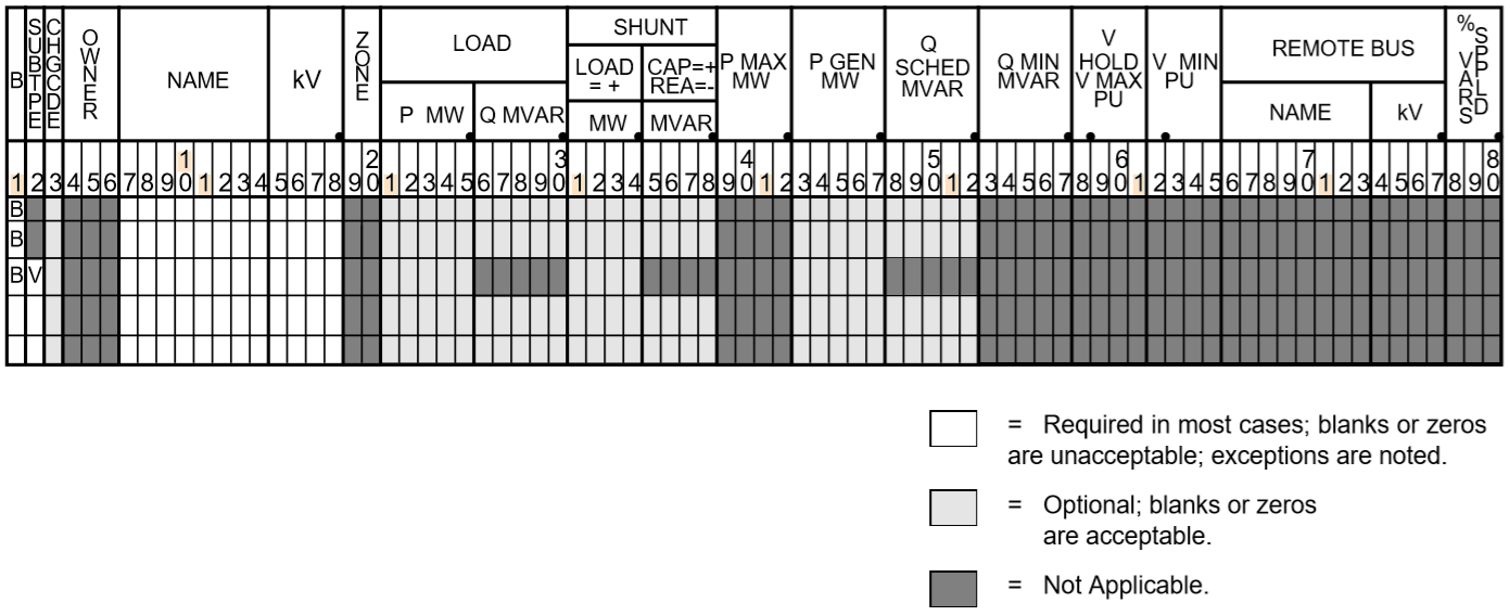
The individual AGC units are identified with type B (bus) records which follow the /AGC command. columns (1:18) correspond with the original format. Beyond column 18, data is free field.
Pmin Minimum generation in MW. Default value is 0.0.
Pmax Maximum generation in MW. Default is Pmax, which is specified on the bus record.
Pgen Base generation is MW, which is used to compute the excursions. Default is scheduled or actual MW from the base case.
% Percentage. The default allocates% in proportion to Pmax
A maximum of 24 AGC units may be specified. One of the units must be a system or area slack bus. Usually, AGC schemes converge faster than non-AGC. The exception occurs when Pmin or Pmax limits are hit and some readjustment occurs.
In Case 2, we apply AGC with 50% on each machine. Presuming that losses are unchanged (for simplicity), the initial and final values are shown in the table below.
Notes and Restrictions
A maximum of 24 generators are permitted. One of the generators must be a system slack bus or an area interchange bus. Recall that the dynamics which drive AGC comes from slack bus P excursions.
If any unit hits a limit, the remaining active units redistribute their percentages and continue AGC control.
The results are summarized in the listing AGCControl. This listing is controlled with /ANALYSIS_SELECT command.:
/ANALYSIS_SELECT>SUM%VAR
If area interchange control is ON, all AGC units should reside in the same area. Violations of this rule are flagged with warning diagnostics.
AGC control will obscure the change in slack bus power shown in the tie line Summary of Area Interchange. The true slack bus effects within the area would be the aggregate effects of all AGC units. The area interchange summary obscures this effect.
When /AGC’s and /GEN_DROP coexist, /AGC operates with a higher priority. In actuality, the two should not coexist.
The validity of AGC can be verified in the analysis summary AGCControl. In normal conditions, the scheduled and actual percentage participation should be equal.
If these quantities are not equal, it is usually because Pmax or Pmin limits have been hit. In this instance, a comment appears.
Actual%/Sched%=****.*
All of the active units should have an individual ratio
This selects individual analysis reports for printing or microfiche. It supersedes /F_ANALYSIS and /P_ANALYSIS. Unlike these commands which select groups of reports according to their “level” the /ANALYSIS_SELECT command selects reports individually.
A solitary /ANALYSIS_SELECT command defaults all analysis listings to no print/no fiche status.
Printing and/or microfiche are enabled with the commands: >FICHE and >PAPER. These commands independently restrict the contents of FICHE or PAPER reports to subsets of Zones, Ownerships or Areas.
The desired analysis reports are individually selected using > commands containing abbreviated report names, e.g., >UNSCH.
Each >(report) command accepts an optional F or P qualifier. This will restrict the selected report to Fiche or Print respectively. If neither appear, both F and P are presumed to be selected. For example, >UNSCH,P will print the unscheduled reactive report.
A special option exists on the >LINEFF report. Its entirety is:
This command specifies that the base case will be established from a master branch data file and associated bus data file. Branch data selected from this file will have an energization date (date in) and a de-energization date (date out) corresponding with the DATE specified on the above command.
If BUSDATA_FILE is not specified or has parameter value *, the program expects bus data to follow in the input stream.
See MERGE_OLD_BASE and MERGE_NEW_BASE for more information about branch data file merging. Using the MERGE_OLD_BASE and MERGE_NEW_BASE commands is preferred.
The primary motive of sensitivity is to calculate the instantaneous system response to sudden capacitor switching operations. This is difficult to model in the Powerflow because all LTCs must be turned off. This may cause solution divergence because LTCs are an integral part of any DC system. This problem is circumvented using sensitivities.
By recalculating the Jacobian matrix, various constraints can be changed. The flexibility of these constraints is evident in the format of the sensitivity command.:
The first two options correspond with the standard solution options. The second two options define the conditions in which type BQ and BG buses can operate holding constant voltage.
For example, enabling the option Q_SHUNT=FIXED, type BQ buses have all shunt fixed. If there is no rotating machinery (\(Q_{max}\) and \(Q_{min}\) are zero), then the bus holds constant \(Q\) (\(PQ\)). Since type BG buses always have Q_shunt fixed, this option has no affect on generator buses.
Similarly, by enabling the option Q_GEN=FIXED, type BQ and BG buses have all generation fixed and operate in state \(PQ\). Type BG buses will operate in state \(PQ\). If BQ buses have no shunt, they also will operate in state \(PQ\).
In order of time response, the generators respond within several seconds. Thus, Q_GEN will normally be adjustable. LTC’s, DC LTC’s, and switched capacitors are controlled by time-delayed voltage relays to minimize spurious operation.
LTC’s 0.5 - 3.0 minutes
DC LTC’s 5 seconds
CAP/REACTORS:5 - 30 seconds
The slowest component is area interchange control. Its response time is 0.5 to 10 minutes.
By appropriate selection of options, the Jacobian matrix can represent nearly any time frame of response.
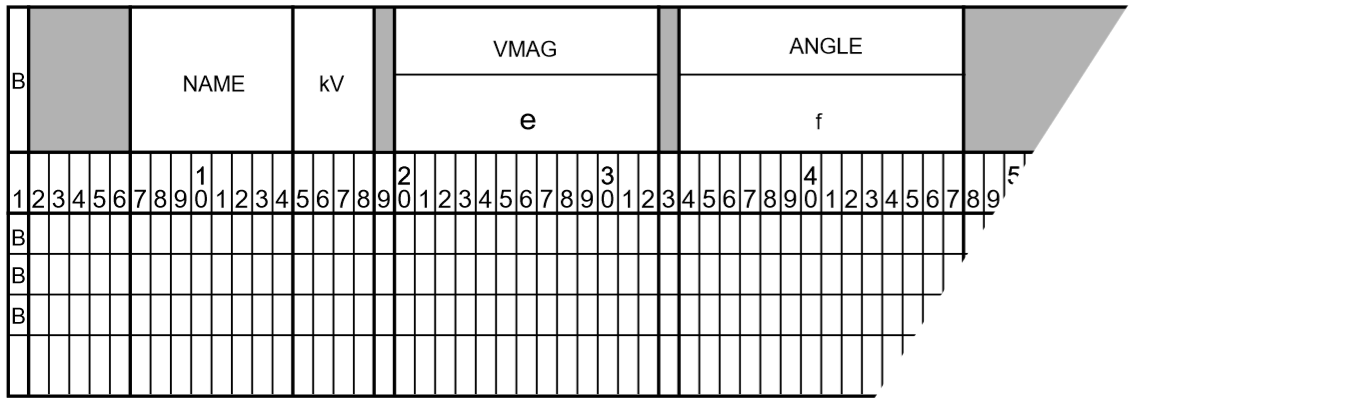
Following the BUS_SENSITIVITIES record, individual buses are selected for perturbation. These buses are identified by the B formatted records that follow them. A maximum of 50 buses may be specified.
The perturbed quantity is identified by nonzero entities in one of the fields: P_load, Q_load, G_shunt, B_shunt, P_generation or Q_generation.
The fields on the B-blank record determine which sensitivity \(\frac{dP}{d\theta}\), \(\frac{dP}{dV}\), or \(\frac{dQ}{dV}\) is computed.
A powerful feature of the sensitivity process is the ability to refactor the Jacobian matrix under different control schemes. For example, one /BUS_SENSITIVITIES record could enable only the Q_GEN option (exciters on, everything else off) for an instantaneous response. Following the necessary B formatted records a second /BUS_SENSITIVITIES record could enable all options for a long term response. Assuming the same bus list is repeated, then a comparison between the two corresponding sensitivities would yield the short-term and long-term effects of the bus’s injection perturbation.
The following is an actual case. Bus OLYMPIA230 was specified for a -172 MVAR shunt application. If Q_Load or Q_Generator was specified, the actual Q_Perturbation would be -172 MVAR. For Q_Shunt, the Q_Perturbation is calculated.:
The correct computed value on the listing is 238.90 kV. The different figures in the example are due to round off.
The correlation with actual Powerflow cases is very close. The calculated voltage excursion -6.54 kV is within two percent of the actual excursion. The accuracy is significant because the actual and estimated voltages will differ 0.001 per unit at most!
This command disables voltage control in selected areas of the system and performs bus type changes from a voltage control type to a more passive type. The changes it makes are permanent and apply to the case in residence. If this command appears before any system changes, the bus type changes will apply before the system changes, exempting any new or changed buses. If this command appears after any system changes, any new or changed buses will be subject to bus type changes invoked with this command.
The LIST parameter accepts two values – ON and OFF. The default is ON. This applies to the CHANGE_BUS_TYPE summary where the initial and final state of each bus affected is depicted. Setting LIST=OFF is recommended for repetitious batch runs.
Means are available to exempt individual buses from type changes defined in the /CHANGE_BUS_TYPE command. These buses are excluded with the following command:
This feature temporarily replaces the ordinary BG -> BC voltage control of a remote bus with a BG control of a compensated voltage, which is specified as a percentage within the step up transformer. This control scheme is valid only for this case, and may be introduced only within context of a CHANGE_BUS_TYPE command. In subsequent cases, these generators revert to their normal control mode
The target compensated voltage is defined with a computed voltage limit. That limit is derived from two base case terminal voltages – the BG bus and the remote BC bus (the remote bus may be another type). The formula used is
This feature is similar to Line Drop Compensation; it temporarily replaces the ordinary BG -> BC voltage control of a remote bus with a BG control of a compensated voltage, which is specified as the voltage drop from the bus terminal voltage computed with the generator reactive power in series with a user-specified impedance. This control scheme is valid only for this case, and may be introduced only within context of a CHANGE_BUS_TYPE command. In subsequent cases, these generators revert to their normal control mode
The target compensated voltage is defined with a computed voltage limit. That limit is derived from two base case terminal voltages – the BG bus and the remote BC bus (the remote bus may be another type). The formula used is
Restrictions on Reactive Compensation
The following restrictions apply to reactive compensation are identical to those which apply to line drop compensation:
All buses selected for Reactive Compensation must be type BG. All buses selected are exempt from any bus type change BG -> BQ or BG => B.
The controlled remote bus must be immediately adjacent to the generator.
The specified percentage is typically in the range 5-6%. It may be negative if the voltage is internal to the machine.
A maximum of 20 generators may be selected for reactive compensation.
The reactive compensation is case specific. It defines the base solution, but is not saved on the base history data file.
Output Reports
A special summary of all line drop compensation buses is listed in the analysis group under the title Summary of Line Drop Compensation. It is available either as a level 4 option on the /P_ANALYSIS or /F_ANALYSIS command or as the SUM%VAR option on the /ANALYSIS_SELECT command.
In this example, the disabling of remote voltage control is restricted to area NORTHWEST. Within this area, all BG generators are permanently changed to type BQ; all LTCs are disabled; and all BX buses are frozen to their discrete value.
This is one of the three commands which are order-dependent on the /SOLUTION command (the other two commands are LINE_SENSITIVITIES and LOSS_SENSITIVITIES). Each of these must follow the /SOLUTION command.
The /CHANGE_PARAMETERS command perturbs a specified network parameter immediately after a successful solution, and initiates a new solution. The process continues until the last /CHANGE_PARAMETERS command has been read. All changed network parameters are permanent in the base case in residence. The output, analysis, and saved base case reflecting the final values of the parameters from the last change.
The /CHANGE_ANALYSIS feature is extremely useful to quickly and accurately generate a set of points for plotting Q-V and P-V curves. When used in conjunction with /USER_ANALYSIS, the values of additional network quantities can be extracted during each /CHANGE_PARAMETERS, enriching the scope of examination into the network.
The distribution VX, VY, etc., designates both the quantity and the axis on the X-Y data file. Default values (V, Q, etc.) are shown in Table 4-6.
Type BX buses selected with this feature emulate the characteristics of mechanically switched shunt capacitors (MSC) controlled by a voltage relay. This voltage relay operates within a voltage deadband (\(V_{min}\), \(V_{max}\)):
If \(V_{min} < V < V_{max}\), then freeze present \(X_{shunt}\) value.
If \(V < V_{min}\), switch in additional capacitor steps or switch out connected reactor steps to raise the voltage, one step at a time.
If \(V > V_{min}\), switch out connected capacitor steps or switch in additional reactor steps to lower the voltage, one step at a time.
For exposition, the feature is called BX Locking. In the absence of this feature, the normal operation is to switch \(X_{shunt}\) one step per iteration to bias the bus voltage to \(V_{max}\).
Only bus type BX buses may be selected for BX locking.
The feature is limited to a maximum of 10 BX locked buses.
This feature can be inserted after any /CHANGE_PARAMETERS command. It defines when BX switching on selected BX buses becomes locked. Once defined, BX locking remains in effect for the duration of the study.
The voltage limits may be temporarily modified for BX locking. The new voltage limits are entered in columns (58:65) in the ordinary manner. These limits are temporary. After the solution, the original limits will be used for analysis reports.
The BX locking feature is not saved on any generated base case.
V-perturbations are applied on V-constrained buses: BQ not at Q-limits, BE and BS types. If the bus type is unacceptable, it is automatically changed to a type BE and a warning diagnostic is issued.
Q-perturbations are applied on Q-constrained buses: B, BC, BT and BQ in state Q_min or Q_max. If the bus type is unacceptable, it is automatically changed to a type B and a warning diagnostic is issued.
P-perturbation can only be applied on P-constrained buses: all types except BS, BD, BM, and area slack buses.
The second form of /CHANGE_PARAMETERS is LOAD perturbation. Either the P_load or the Q_load, or both, may be perturbed a set percentage.
If no ZONES, OWNERS, or AREAS are specified, the percentage change applies to the entire system.
Note that the %P or %Q quantities in the output file correspond to the load that is changed. It may not be the total system load.
The inclusion of OWNERS with either ZONES or AREAS select candidates that are mutually inclusive.
Note that continuation records are accepted here.
For best results, the %LOAD_CHANGE option should be used in conjunction with GEN_DROP. Otherwise, all increase in load is picked up by the area and system slack buses.
The third form of /CHANGE_PARAMETERS is GENERATION perturbation. Either the P_gen or the Q_gen, or both, may be perturbed a set percentage.
If no ZONES, OWNERS, or AREAS are specified, the percentage change applies to the entire system.
Note that the %P or %Q quantities in the output file correspond to the generation that is changed. It may not be the total system generation.
The inclusion of OWNERS with either ZONES or AREAS select candidates that are mutually inclusive.
Note that continuation records are accepted here.
For best results, the %GEN_CHANGE option should be used in conjunction with GEN_DROP. Otherwise, all increase in generation is compensated by the area and system slack buses.
To circumvent the limitations of monitoring a single bus’s V or Q, additional quantities may be monitored using a user-defined analysis file defined with the /USER_ANALYSIS command.
The user analysis file is processed for each encountered /CHANGE_PARAMETERS command. Its output is appended into an output file with subtype .USR_REPORT
In this example, buses in area NORTHWEST with types BQ, BG, and BX were changed to bring about a freeze in voltage control. The /SOLUTION command is a dummy command, introduced to illustrate the position of the pure /CHANGE_PARAMETERS commands. If the bus name following the BUS= keyword has imbedded blanks, insert a pound sign (#), for example, BELL#BPA.
At the conclusion of an ordinary successful solution, the /CHANGE_PARAMETERS records are processed, one by one. The first encounter will internally change the bus type of RAVER500 to BE, if it is another type, and set its voltage to \(V = 1.065 p.u.\) The perturbation will force a new Newton-Raphson solution. The \(Q\) of RAVER is monitored. Its perturbed solved values will be printed out.
Subsequent /CHANGE_PARAMETERS commands will perform additional perturbations.
/ USER_ANALYSIS,FILE=DRB2:[EOFBMJL]USANLINE.DAT
/ CHANGE_BUS_TYPES, BQ=B,BX=B,BG=BQ,LTC=OFF,AREA=NORTHWEST,BC-HYDRO
/ CHANGE,FILE= *
.
.   THIS CASE MODELS THE P-V CURVE FOR THE POST TRANSIENT
.   CONDITIONS FOLLOWING
.   LOSS OF THE COULEE - RAVER #1 500 kV LINE.
.   INSTALL LINE DROP COMPENSATORS ON COULEE
.   500 UNITS AND JOHN DAY
.   AND ALL DALLES UNITS (EXCEPT 115 kV) AND
.   BONNEVILLE (EXCEPT 115 kV)
.   AND CENTRALIA AND CHIEF JOE
.   300 MVAR SVC AT KEELER AND MAPLE VALLEY
.
BGM   CENTRALA20.0
BGM   BONN PH213.8
.
/ GEN_DROP, INIT=75,AREA=NORTHWEST,BC-HYDRO
B       LIBBY    13.8,   PMIN= 289.2,  PMAX=289.2
.
/ SOLUTION
>AI_CONTROL=MON
.
.MONITOR RAVER 500 VOLTAGE AND INCREASE ZONE NA LOAD
.
/ CHANGE_PARAMETERS, BUS = RAVER    500., V = ?
                           %LOAD_CHANGE  %P = 0.5, %Q = 0.5, ZONES = NA
/ CHANGE_PARAMETERS, BUS= RAVER     500.,  V= ?
                           %LOAD_CHANGE  %P = 0.5, %Q = 0.5, ZONES = NA
/ CHANGE_PARAMETERS, BUS= RAVER      500., V= ?
                           %LOAD_CHANGE  %P = 0.5, %Q = 0.5, ZONES = NA
.
.
(END)
If the system is severely perturbed, /CHANGE_PARAMETERS will cause divergence. If this happens, it is assumed that subsequent perturbations will be severe, so divergence will cause them to be ignored. A diagnostic will be issued.
This command introduces comment records into the output report. The comments will appear at the beginning of some output listings. The /COMMENT command is optional; all C comments in the bpf control file will be processed.
Comment text must have a C in column 1. Up to 20 comment records are permitted. Comment text is put in columns 2-80. Comments are saved in any NEW_BASE file for use when getting a plot.
When bpf loads a base file, any previous comments are deleted, then all comments in the bpf control file are added. The result is that only the comments in the bpf control file are saved.
This command combines features of a common mode file used in the CFLOW program pvcurve with the output reports used in the Outage Simulation program, in effect emulating a “slow outage” program. It was written specifically to accept the pvcurve input file without modification.
The outages, defined as MODE within the script in the COMMON_MODE file, typically consists of a sequence of commands /CHANGE_BUS_TYPES, /CHANGES, /SOLUTION, and /GEN_DROP. The mode itself is defined by name on a leading >MODE record; its composition is defined with the change records following a /CHANGES command.
At the end of each >MODE set contaiined within the file named in the COMMMON_MODE command, the solution results (or divergence state) are analyzed: line overloads and bus under/over voltages are written to the user-specified output file in the same format for the OUTAGE_SIMULATION program.
The capability to restrict the analyzed output to subsystems defined with base kV’s and zones as is now done in the OUTAGE_SIMULATION program also exists in this feature. That is the purpose of the OUTAGE_FILE. The OUTAGE_FILE is a bone fide OUTAGE_SIMULATION file which processes only two of its commands: >OVERLOAD and >OUTAGE. All others are ignored. (The >OUTAGE command is used only if the >OVERLOAD commnad is missing and becomes a clone of an implied >OVERLOAD command.)
Initialization phase. The /COMMON_MODE_ANALYSIS record is parsed and the relevant input and output files are opened.
The mail loop to process >MODE records. The base case in residence is reloaded and the associated processes within the >MODE set are processed exactly in the manner performed in the batch powerflow program. At the conclusion of a solution the output results (line overloads, bus under/over voltages, and any solution divergence) are tabulated in interrnal arrays.
At the conclusion of the last >MODE command, the tabulated results are cross-compiled and outputted exzactly in the form as is none in the OUTAGE_SIMULATION program.
This command requests that an analysis report for selected zones or owners be added to the microfiche output file. Note that a separate command [FICHE] must be present in order to save anything on microfiche, regardless of printer and analysis options selected.
When <list> is blank, asterisk, or null, ALL is assumed unless limited by a preceding statement.
The level number determines the analysis summaries to be displayed.
For LEVEL=1, the following summaries are included:
User-defined analysis (optional).
Buses with unscheduled reactive.
For LEVEL=2, the following are displayed with summaries for LEVEL=1:
Total system generations and loads by owner.
System generations, loads, losses and shunts by zones.
Undervoltage-overvoltage buses.
Transmission lines loaded above XX.X% of ratings.
Transformers loaded above XX.X% of ratings.
Transformer excited above 5% over tap.
Transmission system losses.
BPA industrial loads.
dc system.
Shunt reactive summary.
Summary of LTC transformers.
Summary of phase-shifters.
Summary of %Var-controlled buses.
Summary of type BX buses.
Summary of adjustable Var compensation.
Transmission lines containing series compensation.
For LEVEL=3, the following is displayed in addition to the LEVEL=2 output:
Bus quantities.
For LEVEL=4, the following are displayed in addition to the LEVEL=3 display:
Spinning reserves.
Transmission line efficiency analysis. Lines loaded above XX.X% of nominal ratings.
Transformer efficiency analysis. Total losses above X.XX% of nominal ratings.
Transformer efficiency analysis. Core losses above X.XX% of nominal ratings.
This command lists input data on FICHE. Output can be restricted to individual zones specified in <list> and separated with commas. Note that FULL or NONE may be specified in two forms.
The ERRORS option is set to suppress the input fiche if any fatal (F) errors are encountered. This is the default. It can be overridden by setting ERRORS=LIST.
This command lists output on FICHE. Output can be restricted to individual zones specified in <list> which are separated with commas. Note that FULL or NONE may be specified in two forms.
The FAILED_SOL option is set to override the output listing if a failed solution occurs. It defaults to a full listing. A PARTIAL_LIST observes zone lists.
This feature picks up generation from selected generators to balance generation drop. Generation is dropped in one of two ways:
By system changes with the amount specified under INITIAL_DROP.
By PMIN and PMAX limits on selected generators. (These buses are specified with specially formatted B records which follow.)
Generator dropping emulates the short-term characteristics of a system’s response where the generation deficit is automatically picked by other machines. The magnitude is presumed to be proportional to PMAX after the effects of the machine’s transients have damped out.
Candidate generators that pickup are those in the area of interest with a spinning reserve (a surplus of \(P_{max}\) over \(P_{gen}\)). The pickup of an eligible machine “i” is allocated proportionally by the ratio
where \(TOTAL_DROPPED\) is the sum of dropped MW, and \(TOTAL_PMAX\) is the sum of all candidate machines with spinning reserve.
Some machines may be driven to their \(P_{max}\) limits during reallocation. In this case, the allocation becomes nonlinear and several iterations may be required.
A detailed list of each command follows.:
If generation dropping and allocation occurs over several areas, intertie flows may be substantially affected, and it is recommended to change the area interchange from control to monitor unless the new interchange schedule is known.:
One other command also affects area interchange control, the >AI_CONTROL option on the /SOLUTION record. If this follows the /GEN_DROP command above, it may overwrite the selected option.
Generation reallocation continues until the mismatch between generation dropped and generation pickup is less than the tolerance. The default value is 10 MW.
TOL=####
The field #### denotes the numerical values in MW.
The generation to be picked up may be either system-wide (the default) or restricted to a set of areas or zones.
AREAS=<area_1,...>
or
ZONES=<zone_1,...>
The individual areas are separated with a comma (,). If the area name contains a blank, temporarily replace the blank field with a pound sign (#). Continuation records may be employed for aesthetics.
Means are available to contract the system or subsystem defined in the /GEN_DROP command. Individual buses may be excluded from participating in generator pick-up. These buses are selected with the following command:
The amount of generation is defined as the sum of INITIAL_DROP plus the computed generation to be dropped. The computed generation drop is the amount of violation of P-limits on all specified buses:
PMIN<PGEN<PMAX
Obviously, only area and slack buses and AGC candidates permit the P-generation to change. Limits can be placed on these buses by specifying a + or - tolerance, or a PMIN and PMAX (in MWs). PMIN keeps slack buses within a narrow range. The special B records introduce these limits explicitly. This is illustrated with the following example:
BMORRO418.0,TOL=20BMORRO418.0,PMIN=147,PMAX=167
If the key words PTOL, PMIN, or PMAX are omitted, PMAX is taken from the PMAX field on the original or changed bus data record. Recall that on the bus record there is no corresponding field for PMIN. Consequently, PMIN = 0.0. At least one B record must be present.
MORRO 4 is held between 147 and 167 MWs. Dropping 2450 MWs and picking it up elsewhere will change the generation flows and, quite likely, will alter the system losses. The system slack bus accommodates these changes in losses.
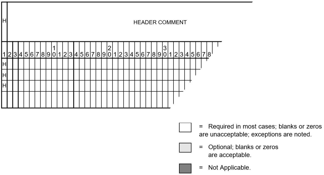
This command introduces one or two header records into the pagination. Its text will be repeated on the top of each page in the output report. Each header record begins with an H in column 1. It is used to supply the lines of text that will be printed at the top of every page of an output listing, below the standard header1, which contains the caseid, project, program version, and date. These header records are saved in the base case file, and any previous headers are deleted. This is similar to the /COMMENT command.
This command permits the input stream containing commands to be temporarily diverted to the named file. Following an end-of-file, control reverts to the normal input stream.
Some restrictions apply. This “included” command file cannot contain any of the following commands:
Use this command to list lines that are loaded above the prescribed LOADING. The output can be filtered by owners. BPA is the default if no owners are specified.
Three commands are dependent on the SOLUTION command. The commands are CHANGE_PARAMETERS, LINE_SENSITIVITIES, and LOSS_SENSITIVITIES. These three work correctly only if they immediately follow the SOLUTION command.
Line sensitivities relate line immittances (impedance or admittance) to voltage, real power flow, and system losses. Six types are available.
\(d\frac{P_{ij}}{dX_t}\) Change in lineflow \(P_{ij}\) with respect to change in transfer reactance \(X_t\) .
\(d\frac{P_{ij}}{dB_s}\) Change in lineflow \(P_{ij}\) with respect to change in shunt susceptance \(B_s\) .
\(d\frac{Loss}{dX_t}\) Change in system losses with respect to a change in transfer reactance \(X_t\) .
\(d\frac{Loss}{dB_s}\) Change in system losses with respect to a change in shunt susceptance \(B_s\) .
\(d\frac{V_i}{dX_t}\) Change in bus voltage (\(V_i\)) with respect to a change in transfer reactance \(X_t\).
\(d\frac{V_i}{dB_s}\) Change in bus voltage (\(V_i\)) with respect to a change in shunt susceptance \(B_s\) .
The change in transfer reactance \(X_t\) or shunt susceptance \(B_s\) pertains to an existing line. The command statement which invokes line sensitivities is:
The top line depicts default quantities. The options LTC and AI_CONTROL pertain to LTC transformers and area interchange control.
The second part of the sensitivities is the perturbed quantities \(dX_t\) or \(dB_s\). They are defined with specially formatted > records and are similar to L records.
>PB: \(\frac{dP_{ij}}{dB_s}\) or \(\frac{dP_{ij}}{dX_t}\)>LB: \(\frac{dLoss}{dB_s}\) or \(\frac{dLoss}{dX_t}\)>VB: \(\frac{dV_i}{dB_s}\) or \(\frac{dV_i}{dX_t}\)
(7:18)
A8,F4.0
Bus1 name and base kV
(20:31)
A8,F4.0
Bus2 name and base kV
A1
Circuit ID
I1
Section number
(45:50)
F6.5
Perturbed \(X_t\)
(57:62)
F6.5
Perturbed \(B_s\)
A maximum of 50 perturbed quantity > records may be present.
The ambiguity \(d(.)/dB_s\) or \(d(.)/dX_t\) is resolved by non-zero entities for \(X_t\) or \(B_s\) . If both are zero, the default is \(X_t\) . Non-zero entities define the magnitude of the perturbed quantity \(Delta X_t\) or \(Delta B_s\). Perturbed flows, losses, or voltages will be computed using these values.
The perturbed branch flows \(P_{ij}\) are identified with the individual L records that follow. If parallel lines are present, \(P_{ij}\) pertains to the total of all parallel flows.
The perturbed voltages are the 20 largest excursions effected by the change in immittance. The perturbed losses are a simple quantity. An example setup follows:
The first perturbation >PB with blank \(X_t\) and \(B_s\) fields requests \(\frac{dP_{ij}}{dX_t}\) (the default). The individual \(P_{ij}\) records.
The second perturbation >LB with blank \(X_t\) and \(B_s\) fields requests \(\frac{dLoss}{dX_t}\) (the default). No L records follow because the monitored quantities are system losses.
The third perturbation >VB with blank \(X_t\) and \(B_s\) fields requests \(\frac{dV_i}{dX_t}\) (the default). No L records follow because the monitored quantities are perturbed voltages. The 20 largest excursions are listed.
This set of commands automatically converts constant power, constant current, or constant impedance loads to a user-specified distribution of constant MVA, constant current, and constant impedance.
The option DISTRIBUTED_VOLTAGE (or DIST for abbreviated form) selects either NOMINAL (all voltages are 1.0 p.u.) or BASE, which is the individual bus’s voltage.
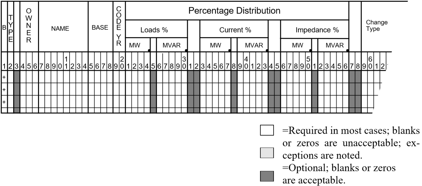
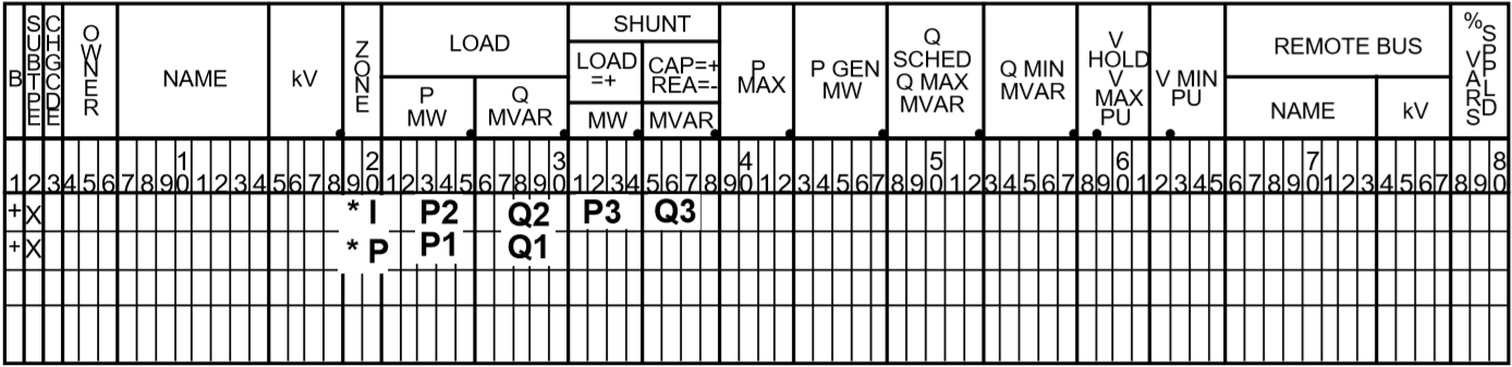
Constant current loads and constant impedance loads are defined by continuation bus (+) records using reserved TYPE s and CODE_YR s. Constant impedance loads differ from \(G_{shunt}\) and \(B_{shunt}\) quantities in the sense that these quantities are converted into loads and appear in special analysis summaries. The table below describes these special codes and their interpretations.
For expositional purposes, we will call constant current \(A_{load}\) and \(B_{load}\). This nomenclature is consistent with the expression for complex current:
\(I = A + jB\)
The power at a constant current load is computed with the expression
\(P_{load} + jQ_{load} = complx( V ) * conjg( I )\)
where \(complx(V)\) is the complex voltage and \(conjg(I)\) is the conjugate of the complex current. The use of the conjugate expression is needlessly complicated for this simple application and has been relaxed. The quantity Bload is stored as its conjugate, that is, no sign reversal is needed to interpret the correct sign of the load in MVAR.
Let \(V\) denote the per unit base or nominal voltage magnitude - depending upon the option DISTRIBUTED_VOLTAGE. The distributed constant current loads in MW and MVAR are computed as follows:
Readers may note that this is not true constant current. True constant current loads involve the system phase angle. The modelling here is more lenient: it is constant power factor.
The negative sign for \(B_{shunt}\) is correct. The actual expression is
\[P + jQ = conjg (Y) * V^2\]
A positive value of \(G_{shunt}\) is the same sign as load; a positive value of Bshunt is the same sign as generation.
Those buses whose loads can be distributed can be selected either individually or systematically. Individually selected buses require the >CHANGE_BUSES command. Systematically selected buses require the >CHANGE_SYSTEM command.
>CHANGE_SYSTEM,PLOAD=##% P + ##% I + ##% Z,QLOAD=##% Q + ##% I + ##% Z,AREAS=area_1....,ZONES=zones_1,...,OWNERS=owner_1,>EXCLUDE_BUSESBnamebaseBnamebaseBnamebase
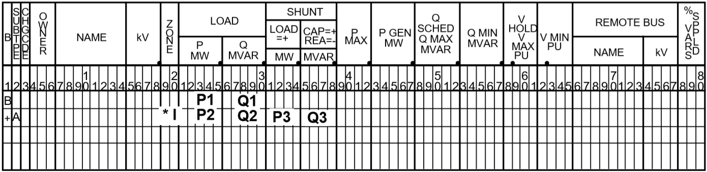
This example redistributes constant power loads according to the specified percentages.
The redistributed constant current and constant impedance loads are transferred to a new +A01 continuation bus record. The redistributed constant power loads replace the original constant power load.
A special feature has been added to redistribute constant current and constant impedance loads that already have been distributed. As such, these loads are restricted to +A01 and +A02 continuation bus records. The table below describes these options.
Table 45 Constant Power, Current, and Impedance Keywords
Type of Load to Convert
Keyword for Real Part
Keyword for Reactive Part
Constant Power
PLOAD =
QLOAD =
Constant Current
ALOAD =
BLOAD =
Constant Impedance
RLOAD =
XLOAD =
For example, to change constant current loads, the following commands are used:
>CHANGE_SYSTEM,ALOAD=##% P + ##% I + ##% Z,BLOAD=##% Q + ##% I + ##% Z,
The network affected by the specified load change percentages can be restricted to buses within a given subsystem. This subsystem can be defined by those buses having common attributes in two sets:
{AREAS,OWNERS}
or:
{ZONES,OWNERS}
ZONES and AREAS are mutually exclusive; only one of the above can be specified.
If no owners are specified, all ownerships are implied. The selected subsystem can be further defined by excluding specific bases with the >EXCLUDE option.
More than one set of CHANGE_SYSTEM commands is permitted. This would permit buses in different areas or zones to have different percentage distribution factors. In case of overlap, precedence is given to the first definition.
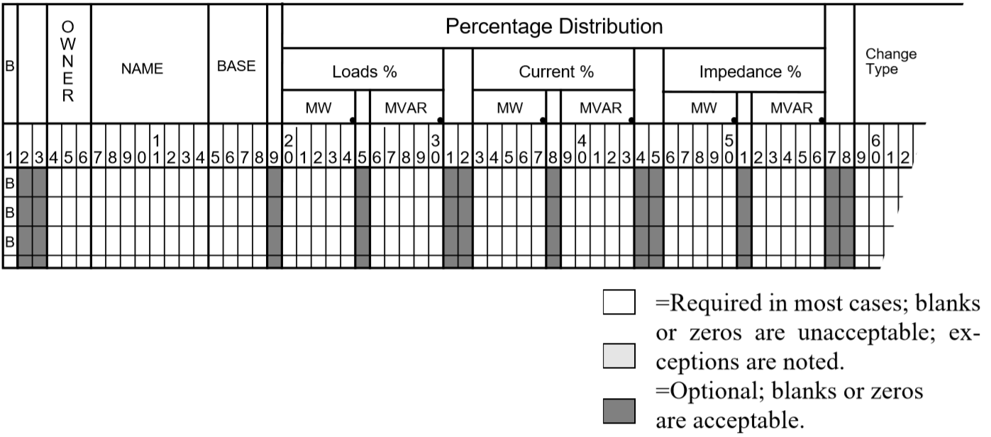
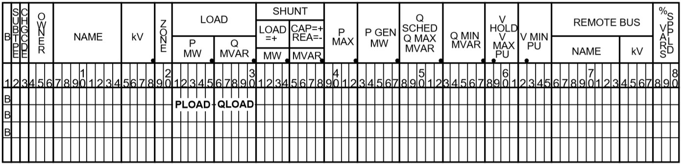
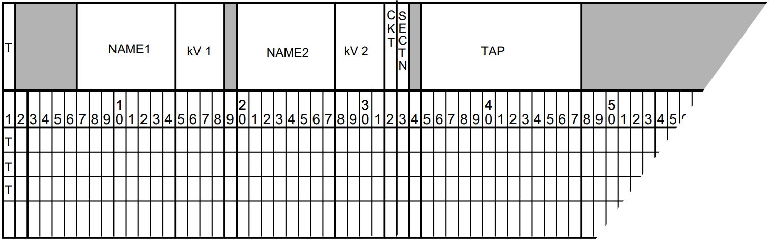
This command permits unique distribution factors to be specified for individual buses. The buses and their distribution factors are identified on fixed field records. The format of the B % load change record is shown in the figure below. CHANGE_TYPE is optional. ALOAD and RLOAD have the same interpretation given in Table 4-8. Thus, they would apply to + records, but not to B records.
If the ownership field is blank or includes the bus ownership, the percentages apply only to data on the bus B record. Continuation bus data will not be affected.
On the other hand, if the ownership is the magic code ###, the percentages apply to data on the bus B record and also to data on all associated continuation bus records.
Fig. 58 CHANGE_BUS % Load Input Format for B Records
If separate % changes are to apply to bus and continuation bus records, separate +% change records must be used—one for the bus B record and others for the specific + bus records.
The identification fields for +% bus records are identical to those for the + records as in the table below.
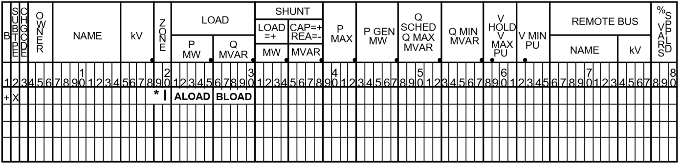
ALOAD, BLOAD distributions applied on a +X*P bus record.:
ALOAD=%PL+%PI+%PZBLOAD=%QL+%QI+%QZ
Note that ALOAD and BLOAD quantities are generated by prior %LOAD_DISTRIBUTION. Thus, this record corresponds to a + record having the same TYPE and CODE_YEAR. See below.
The load distribution is presumed to apply to a solved base case. At the base solution, the total load in MWs and MVARs is unchanged after distribution. If the system is not otherwise changed, the solution should converge to the base solution.
Each nonzero load on a bus or continuation bus record generates an associated constant current and constant impedance load on an equivalent +A*I continuation bus record.
The continuation bus array is currently dimensioned for 3360 records.
The number of generated +*I and +*P records in a typical base case averages 400 (assuming one for each continuation bus) plus one for each number of nonzero load on the bus records.
BPA’s Transient Stability Program in its present form cannot accommodate the Powerflow model of constant current loads.
This qualifier introduces a reference base case from which to derive missing ownership and mileage information. The GE data set is potentially richer in content than IPF’s base data file, but maybe incomplete if some optional data fields such as mileage or ownerships are omitted.
VERSION=<nnn>
This qualifier defines the version number of the input data. At present, only version 21 is recognized.
RATINGS=(TX=AABC,LN=AAC)
This option correlates the various GE branch ratings with the IPF branch ratings. Four GE transformer ratings (RATEA, RATEB, RATEC, RATED) can be assigned independently to the IPF transformer ratings in the following order – Nominal, Thermal, Emergenty, and Bottleneck, Simarily, three GE line ratings (RATEA, RATEB, RATEC) can be assigned independently to the IPF line ratings in the following order – Nominal, Thermal, and Bottleneck.
The default branch IPF ratings, shown in the example above, are assigned per the table below.
This option defines the remotely controlled bus’ voltage assignments in the form of bus type and scheduled voltage. The table below describes all options
Table 47 Remotely controlled bus assigned voltages
This qualifier introduces a reference base case from which to derive missing ownership and mileage information.
VERSION=<nnn>
This qualifier defines the version number of the input data. At present, only version 3 and 4 are recognized.
RATINGS=(TX=AABC,LN=AAC)
This option correlates the various PTI branch ratings with the IPF branch ratings. Four PTI transformer ratings (RATEA, RATEB, RATEC, RATED) can be assigned independently to the IPF transformer ratings in the following order – Nominal, Thermal, Emergenty, and Bottleneck, Simarily, three PTI line ratings (RATEA, RATEB, RATEC) can be assigned independently to the IPF line ratings in the following order – Nominal, Thermal, and Bottleneck.
The default branch IPF ratings, shown in the example above, are assigned per the table below.
This option defines the remotely controlled bus’ voltage assignments in the form of bus type and scheduled voltage. The table below describes all options.
Table 48 Remotely controlled bus assigned voltages
Three commands are dependent on the SOLUTION command. The commands are CHANGE_PARAMETERS, LINE_SENSITIVITIES, and LOSS_SENSITIVITIES. These three work correctly only if they immediately follow the SOLUTION command.
This feature provides valuable information concerning system losses with respect to scheduled active and reactive generation or loads, and to scheduled voltages. The command statement that invokes loss sensitivities is:
The top line depicts default quantities. The options LTC, AI_CONTROL, and Q_SHUNT pertain to LTC transformers, area interchange control, and \(B_{shunt}\) on type BQ buses.
Three loss sensitivities are computed: \(\frac{dLoss}{dP_i}\), \(\frac{dLoss}{dQ_i}\), and \(\frac{dLoss}{dV_i}\).
These sensitivity computations are linearized about the solved case. For small changes, the sensitivities are extremely accurate. For larger changes, non-linearities redefine the problem. A rule of thumb is that the sensitivities are sufficiently accurate for a 0.5 per unit (p.u.) change in \(P_i\) or \(Q_i\), and a 0.01 p.u. change in \(V_i\).
Each sensitivity relates changes in the system losses to a hypothetical change of 1.0 p.u. in scheduled active generation \(P_i\), reactive generation \(Q_i\), or voltage \(V_i\).
Ordinarily, a decrease in system losses is anticipated when \(P_i\), \(Q_i\), or \(V_i\) increases, that is, a negative loss sensitivity.
An exception often occurs for \(\frac{dLoss}{dP_i}\). Occasionally, \(\frac{dLoss}{dP_i} > 0\), that is, increasing the generation \(P_i\) increases the losses!
Recall the constraint for Area_i:
Areaexport=Areageneration-Areaload-Arealosses
(Any active bus shunt \(G\) is presumed to be accounted for in area losses.)
Within each area, the generation on the slack bus is adjustable and on all other generators is fixed. Thus, a change of 1.0 p.u. on generator “i” causes two changes in the area slack bus:
An immediate transfer of -1.0 p.u. to balance the change in generation.
An additional change to reflect the change in system losses, which are affected by the 1.0 p.u. generation transfer.
Note that the system slack bus or area interchange slack bus must pick up any deficit generation needed to supply loads and system losses. Thus, the sensitivity reflects the change in losses if 1.0 p.u. MW of generation is moved from bus “i” to the system or area slack bus. If the system or area slack bus is closer to the load center, the losses will decrease with the reallocation. Consequently, \(\frac{dLoss}{DP_i} < 0\). Otherwise, the losses will increase.
A change in reactive generation is quite different from a change in active generation. Changes in reactive generation strongly affect the voltage profile of the system adjacent to bus “i”. Thus, a change in losses is due primarily to the change in voltage profile.
A change in scheduled voltage for types BE, BS, BQ, or BG buses directly affects the voltage profile of the system adjacent to bus “i”. Thus, the change in voltages directly affects system losses. In general, higher voltages are accompanied with lower branch currents and hence, lower line losses. Exceptions may occur in cables where large amounts of inductive shunt are necessary to compensate for the capacitance in cable.
These subprocesses extract a subsystem from an old base file and merge it with another subsystem to generate a new system. The subsystems are defined by various qualifiers following the MERGE command.:
file_spec is the file specification for the pertinent file. If file_spec has the value * for either the BUS_DATA_FILE or BRANCH_DATA_FILE, the data is presumed to be the Powerflow command file.
subsystem_label is the identifying label for the merged subsystem.
DATE is the branch extraction date. Branches selected will have their energization date on or before DATE and a de-energization date after DATE.
The month field (as a digit) also defines winter or summer extended ratings:
For other values, it is necessary to use an additional parameter R defined in the next section.
R specifies extended ratings from the branch data file. See Table 4-15 and Table 4-16. Also, see Figure 4-11 and Figure 4-12. Two modes of operation are available:
** Merge a subsystem from one OLD_BASE file with another subsystem from a different old base file.
** Merge a subsystem from an OLD_BASE file with another subsystem which is newly created from bus and branch records.
The two merge control cards distinguish the source of the subsystem data. /MERGE_OLD_BASE identifies an OLD_BASE file, and /MERGE_NEW_BASE identifies the bus and branch records files from which a new subsystem will be constructed.
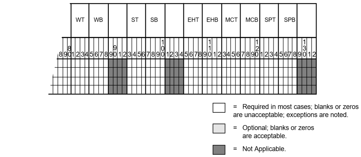
The R code indicates which extended ratings from the branch data file should be used. For example, the R=2 code in the following card indicates that extra heavy ratings should be used.
Powerflow uses appropriate ratings from the branch data for the peak winter (R=1), peak summer (R=8), extra heavy (R=2), moderate cold (R=3), and spring (R=4) choices.
If the thermal or bottleneck rating on a branch is blank or zero in the columns for extra heavy or moderate cold ratings, the peak winter rating is used (if available). Similarly, if the thermal, bottleneck, or emergency rating on a branch is blank or zero in the columns for spring ratings, the peak summer rating is used (if available).
The chosen ratings are moved to columns 81 through 92 on the branch record in Powerflow.
Fig. 64 Extended Ratings Fields for L and E Records
Table 49 L and E Record Extended Fields Column Descriptions
Column
Rating (“R” Selection)
Field Description
81-84
1
Winter Thermal (WT)
85-88
1
Winter Bottleneck (WB)
89-92
(not used)
93-96
8
Summer Thermal (ST)
97-100
8
Summer Bottleneck (SB)
101-104
(not used)
105-108
2
Extra Heavy Thermal (EHT)
109-112
2
Extra Heavy Bottleneck (EHB)
113-116
3
Moderate Cold Thermal (MCT)
117-120
3
Moderate Cold Bottleneck (MCB)
121-124
4
Spring Thermal (SPT)
125-128
4
Spring Bottleneck (SPB)
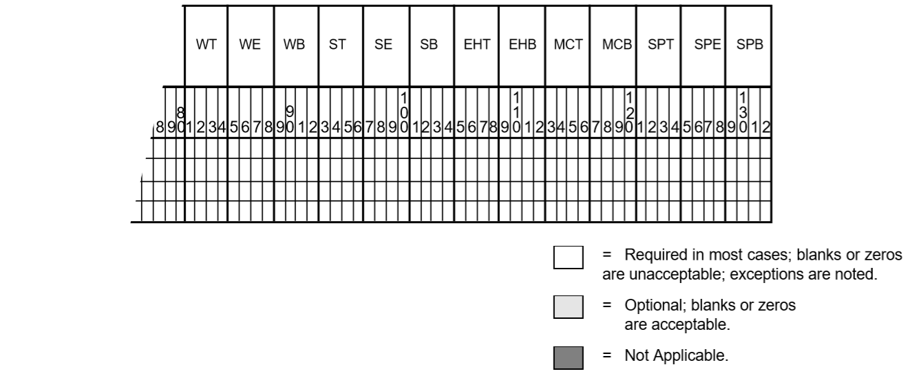
Fig. 65 Extended Ratings Fields for T and TP Records
Table 50 T and TP Record Extended Fields Column Descriptions
Column
Rating (“R” Selection)
Field Description
81-84
1
Winter Thermal (WT)
85-88
1, 2, 3
Winter Emergency (WE)
89-92
1
Winter Bottleneck (WB)
93-96
8
Summer Thermal (ST)
97-100
8
Summer Emergency (SE)
101-104
8
Summer Bottleneck (SB)
105-108
2
Extra Heavy Thermal (EHT)
109-112
2
Extra Heavy Bottleneck (EHB)
113-116
3
Moderate Cold Thermal (MCT)
117-120
3
Moderate Cold Bottleneck (MCB)
121-124
4
Spring Thermal (SPT)
125-128
4
Spring Emergency (SPE)
129-132
4
Spring Bottleneck (SPB)
MERGE qualifiers
>EXCLUDE_BRANCHES
Use this command to exclude from the subsystem branches following this statement. Each branch is identified with a separate L, E, or T formatted record.
>INCLUDE_BUS
Use this command to identify additional buses which are to be included in the selected subsystem. Each bus is identified with a separate B formatted record.
>INTERFACE_BRANCHES
Use this command to list individual interface branches. Each such interface branch is identified with a separate L, E, or T formatted record.:
>INTERFACE_PREF=COMPREJECTACCEPT
This command assigns preference weights on competing interface branches listed following the statement. Two subsystems to be merged are usually topologically complementary and have common branches. These branches are called interface branches. During merging, two sets of competing interface branches vie for selection in the final system. In the absence of any information supplied, the default decision is to select the interface branch with the most detail.
The command above allows the user to assign preferences for the interface branches for each system. Each such interface branch is identified on a standard L, T, or E formatted record. ACCEPT and REJECT must complement each other, or both sets of interface branches will be accepted or rejected.
COMP forces comparison of common interface branches from the two subsystems. Acceptance from one subsystem and rejection from the other is determined on the basis of matching bus and branch ownerships. The assumption is that the bus owner always has better branch data. For BPA users, WSCC data is accepted when branch ownerships cannot be determined from data.:
>MERGE_RPT=SORTEDUNSORTED
This command requests the specific level of merge report. This feature is not yet implemented.
>RENAME_BUS
This command provides a convenient way to resolve potential conflicts of identically named but topologically distinct buses. This command introduces B-formatted records with the old name in columns 7-18 and the new name in columns 20-31.
>SAVE_AREAS
Use this command to save areas of the subsystem listed following this statement. Each area is identified with a separate A-formatted area record.
>SAVE_BASES<list>
This command saves buses whose base kV’s match the list. Elements of the list are separated by commas (,) and terminated by a period (.).
>SAVE_BUSES
This command saves listed buses of the subsystem. Saved buses are named on separate B-formatted bus records following.
>SAVE_ZONES<list>
This command saves listed zones of the subsystem. Elements of the list are separated with commas. Example: >SAVE_ZONESNA,NB
>USE_AIC
This command specifies that A records should be generated from the old base file defined by the OLD_BASE statement.
This introduces network bus and branch data into the program. No old base case is in residence. RXCHECK=ON enables \(R/X\) ratios checking.
If the FILE parameter value is asterisk (*), then bus and branch data is assumed to immediately follow this command.
This command defines the name of the new base file to save the network solved by the case run. It may be the same as the old base file, if you want to overwrite it.
This command specifies that a previously solved Powerflow case is to be loaded from the specified file and used as the base system for the current request.
<filespec> The file specification of the solved network to be re-solved.
The REBUILD switch causes the program to rebuild all of the tables and starts the solution with a “flat start.”
This command simulates the effect of line outages, load dropping, generator outages, and generator rescheduling. It invokes a process which modifies the base case data in residence. For this reason, this process should not be used with any other process.:
This command specifies the threshold loading of a line to be included as contingency-caused overloads. This threshold may be raised on individual branches to screen out base case overloads.:
>COMMON_MODE,FILE=*>COMMON_MODE_ONLY,FILE=*
These two commands introduce a script which defines one or more “common-mode” outages. The second form restricts the outage simulation study to include only common mode outages. In this case, it is still necessary to introduce an associated >OUTAGE record, but it is used only to define the zones and bases of interest.
The simulation and analysis of any common-mode outages complements in a seamless fashion that for the ordinary single-contingency branch outages. The script associated with the common mode study can be either in a separate file (in which case a file name would be specified) or in the input stream (in which case a file name * is specified).
Each common-mode outage consists of two parts: A common-mode identification record (>MODE) and the set of WSCC-formatted bus an/or branch changes which are associated with that common mode outage. It is useful and recommended to annotate this script with comment text. An example will illustrate all the points mentioned.:
Here, the name of the introduced common-mode outage is “B/D DRISCOLT 230”. The name is arbitrary; it should be sufficiently distinct to contrast it with entities associated with ordinary single contingency branch outages. The name is 40-characters long, is defined in columns (7:47) on the >MODE records, and is truncated to 31 columns in certain Outage Analysis listings where it must compete with the single contingency branch outages. A maximum of 50 >MODE records are permitted.
Each >MODE record is accompanied with an set of arbitrary change records which specifically define all of the changes in the system that are effected by the common mode. If no change records are submitted, the >MODE record is meaningless, since it would not perturb the system in any manner.
The common mode changes permitted are restricted to the following:
Bus deletion (D) and modification (M).
Continuation bus deletion (D) and modification (M).
Branch deletion (D).
The change methodology is identical with that used elsewhere. A bus deletion, for example, automatically deletes all components associated with it. Implementation, however, expedites the change, but in a manner designed to maximize the computational efficiency. The same bus deletion, to repeat the example, is effected by temporarily changing the impedance of all emanating branches to 10000.0 p.u. X, and preserving a small residual admittance for the bus.
With judicious selection of change records, it is possible to simulate complex scenarios such as the loss of switching CAPs followed with the loss of a transformer.
If the common mode changes isolate even a single bus in the system, the outage is skipped and the isolation is noted within the outage analysis reports.
Although every attempt was made to simulate common mode outages as efficiently as possible, the highly efficient line compensation schemes that were utilized in the single contingency branch outages could not be used here. Each common mode outage requires refactorization of the associated network matrices.
>DEBUG=OFFON
This turns on debug dumps.
Note
Caution! These dumps can be enormous.
>DEFAULT_RATING
This command indicates that the following text is line default data. Branches in the specified areas of interest are examined for zero rating (which is an omission of data). If the base kVs of the terminals match the kV in the following default ratings, new ratings are assigned to their branches. They then become candidates for branch overload checking following an outage.
See the table below for the format of default ratings.
This command specifies that all line resistance in the eliminated system is replaced with equivalent current injection. The equivalent network, as modified by this option, is easier to solve.:
>EXPAND_NET=2<nn>
This command specifies that the border of the selected equivalent network should emanate outwards an additional number of buses. The expansion selected should be less than 100.:
>GEN_OUTAGE=NONE<nn>
This command specifies the maximum number of generator outages for rescheduling.
>INCLUDE_CON=<filespec>
Use this command to divert the input stream to an auxiliary file that contains /OUTAGE_SIMULATION text. This auxiliary file cannot contain a recursive /INCLUDE_CON statement.:
>LOW_VOLT_SCREEN=80<num>
This command specifies a contraction for overload values to compensate for effects of voltage changes. It lowers the threshold which tests for overloaded lines.:
>MIN_EQUIV_Y=.02<num>
This command specifies minimum admittance of equivalent branches.:
>NO_SOLUTION,ANGLE=3.0,DELTA_V=.5<num><num>
This command specifies conditions for no solution (or no convergence). ANGLE is the largest excursion angle (from one iteration to another) in radians relative to the slack bus.
>OLD_BASE=<filespec>
<filespec> is file specification of the solved network to be re-solved.
Because /OUTAGE_SIMULATION is a stand-alone process, it must begin by loading an old base file which is introduced using this command.:
>OUTAGE,ZONES=*BASES=*<list><list>
This command specifies the ZONES and voltage levels where outages should be taken. Elements of the list should be separated by commas.:
>OUTPUT_SORT,OVER_OUTOUT_OVER,OWNERBOTH
This command specifies the sort order for output listing in terms of overloads and associated outages. The OWNER option requests ownership-bus sort order.:
>OVERLOAD,ZONES=*BASES=*<list><list>
To specify zones and voltage levels where overload should be monitored, use this command. Entities in list should be separated by commas.:
>PHASE_SHIFT=FIXED_POWERFIXED_ANGLE
This command specifies phase-shifter representation constant branch power or constant phase shift angle.:
>REACTIVE_SOL=ONOFF
This command invokes the reactive solution feature. Normally, only the P-constraints are held.:
>REALLOCATE=NONELOADLOADGEN
This command specifies that load may be shed, generation changed, or both, in order to relieve overload.:
>REDUCTION=NONE,REI=OFFSIMPLEONOPTIMAL
This command requests the reduction feature and specifies the type of reduction.:
>REDUCTION_DEBUG=NONEMINORMAJOR
This is used to request the debug feature.:
>RELAX_BR_RATE=ON,PERCENT=5.0OFF<NUM>
This command requests that the branch ratings be relaxed by a certain percentage.:
>SET_RATINGS,NOMINAL,FILE=<filespec>SUMMERWINTER
This command specifies the special ratings of branches that are used for overload determinations. The number of branches whose ratings are specified in FILE is given by a records parameter. Specification records follow this qualifier if the file parameter is omitted. Rating records are described in the table below.
This command sets the solution iteration limit per outage. Divergence is assumed when this limit is exceeded.
>TOLERANCE=.005<num>
This specifies the convergence tolerance in per unit power. Convergence is assumed when mismatch is less than this value. Larger values (0.05) yield fast, approximate solutions; smaller values yield slower, more exact solutions.
The following method has proved to be a useful tool for debugging the Outage Simulation Program (OSP) interactively. In invoking this option, three events occur.
After the equivalent reduced system is established but before the individual branch outages are taken, the user interactively selects from the full set of branch outages one or more outages. The unselected outages will be ignored.
Debugging switches are turned on.
Salient process and status information about each outage is displayed on the screen.
This is most useful to confine the study to a single questionable outage which them will to be compared with the results of an IPF change case depicting the same outage. To invoke this, enter the two following DCL commands in a terminal window.:
$ DEBUG_OUTAGE_SIMULATION_STUDY :== ON
$ RUN IPF_EXE:FSTOUT.EXE_V321
The second command executes the OSP interactively. After responding to the prompted Power Flow Control file and waiting a few minutes, OSP’s special debugging in invoked.
Enter outage range (n:m), 0=Save, -1=Cancel)
You must select the outage by trial and error using a binary search. Enter a candidate outage branch index (say 127). The dialog continues (using an actual case for an example).
127 outage BELNGM P 115.0 CARILINA 115.0 1 : Select? (Y or N)
Selecting “Y” will add this to the outage set’ “N” will ignore it. If the displayed outrage is alphabetically lower than the desired outage, respond with “N” and enter a higher outage number at the next prompt. If it is higher do the opposite. The dialog loops for additional selections or searches.
Enter outage range (n:m), 0=Save, -1=Cancel)
Eventually, when the desired ouages(s) is (are) selected, the process is exited with either option (“0”, saving the selection and continuing or “-1”, ignoring the selection and continuing).
This command lists input data on PAPER. Output can be restricted to individual zones specified in <list>, which are separated with commas. Note that FULL or NONE may be specified in two forms.
The ERRORS options can be set to NO_LIST to suppress the input listing if any Fatal (F) errors are encountered.
This command lists output on PAPER. Output can be restricted to individual zones specified in <list>, which are separated with commas. Note that FULL or NONE may be specified in two forms.
The FAILED_SOL option is set to override the output listing if a failed solution occurs. It defaults to a full listing. A PARTIAL_LIST observes zone lists.
This command requests that all internal data tables be rebuilt using the current specified OLDBASE file. This has the same effect in a case as the REBUILD parameter on the /OLD_BASE statement.
This command reduces the network in residence to a desired size and solves the reduced network. It can be saved or processed further as an ordinary base case. For more detail on the methods used, see Network Reduction.:
This identifies row-coherent generators (or load) of an REI subsystem. The name must be unique, containing 1-7 characters without blanks and be left-justified. The REI components, which will have their generation and/or load transferred to the coherent generator, are identified with ordinary WSCC-formatted bus (Type B) records which follow.
The named constituent buses which comprise each coherent cluster may be either retained or eliminated buses. In either case, the constituent buses will be eliminated.
Special codes on each bus permit individual dispositions of generator and load quantities. Generation and/or load may be converted to constant current, constant admittance, or converted to an REI coherent unit. The codes are show in the table below.
This command determines how the nodal generation, load, and shunt admittance on eliminated nodes is to be processed. It does not affect the original quantities of the interior or envelop (border) nodes. The disposal options are to convert selected quantities to nodal current, to nodal shunt admittance, or to append them to an REI node.
>ENVELOPE_BUSES=BE
This command, when elected, changes the subtypes of all envelope node to type BE. Its primary merit is to secure the voltages of the terminal buses at their base case values an improve the solvability of the reduced equivalent system. The default option is to leave the envelope buses in their original subtype.
>EXCLUDE_BUSES
This command excludes from the retained network the buses listed on the bus-formatted records following this statement. Its purpose is to allow more flexibility in the definition than allowed with a simple SAVE_BASES or SAVE_ZONES. Obviously, the retained system must already be defined by a prior SAVE_BASES or SAVE_ZONES command.
>INCLUDE_BUSES
This command includes in the retained network additional buses listed on the bus-formatted records following this statement. Its purpose is to allow more flexibility in the definition than allowed with a simple SAVE_BASES or SAVE_ZONES. Obviously, the retained system must already be defined by a prior SAVE_BASES or SAVE_ZONES command.
>INCLUDE_CON=<filespec>
Use this command to include a set of user-specified default command qualifiers, which is stored in a file. Such a default command file should not contain this / INCLUDE_CON statement.:
>KEEP_AI_SYS=ONOFF
This command requests that the equivalent network will retain all of the attributes of area interchange control. This includes all area slack nodes and all tie line terminal nodes.:
>MIN_EQUIV_Y=.02<num>
This command specifies the minimum admittance of equivalent branches that are retained. Its purpose is to reduce the large number of equivalent branches which are generated, some of which have such large impedances that their contribution to the flows are marginal. A smaller value of 1.0 is recommended. Equivalent branches which have lower admittances (or what is the same, higher impedances) will be replaced with equivalent shunt admittances at both terminals.:
>OPTIMAL_REDU=ONOFF
This command switches the optimal network determination feature, which precedes the actual network reduction. When the optimal network selection is ON, it may enlarge the user-specified retained system with optimally selected nodes such that the overall size of the reduced system will be minimized. In essence, it expands the boundary into the eliminated system in a manner which will topologically result in an equivalent network having more buses but fewer branches overall. Thus, the user defines a fuzzy retained system containing the minimum desired configuration, and the optimal network selection will enlarge the network if feasible.:
>RETAIN_GEN=OFF,PMIN=100.0ON<num>
This command selected all generators with generation > PMIN to be in the retained network.:
This command works in conjunction with the REI option on the ELIM_MODE command. An attempt is made to automatically consolidate REI clusters which may have only a single node. However, their consolidation may result in an equivalent REI node whose voltages are too bizarre. It is electrically correct, but may cause solution problems since voltages are initialized about 1.0. By restricting the voltage differences of REI consolidation candidates to those whose voltage differences are less than the user-prescribed value, the resultant consolidated REI cluster will have a more feasible voltage.:
>SAVE_BASES=<list>
This command defined the retained network as consisting of those buses which have the base kvs in list. Elements of list are separated with commas (,).:
>SAVE_BUSES
This command defines the retained network as consisting of all buses identified on the following bus-formatted records. It is a brute force method to define the retained network. It cannot be used in conjunction with SAVE_ZONES or SAVE_BASES. See INCLUDE_BUSES.:
>SAVE_ZONES=<list>,BASES=<list>
This command defines the retained network as consisting of those buses which have zones in the first list, with the optional, additional provision that their base kvs must be in the second list. Elements of the list are separated with commas (,).:
>STARTING_VOLTAGES=FLATHOT
This command defines the starting voltages which will be used in the ensuing rebuilding and solution of the reduced equivalent base. The default is FLAT, meaning that the solution will use flat starting voltages. There are two separate applications for this option.
The first application is to verify the integrity of the equivalent bus and branch data structures from the complex reduction processing. When used in conjunction a another solution option:
/SOLUTION>BASE_SOLUTION
the ensuing convergence checks performed in output report independently verify the validity of the reduced bus and branch data.
The second application is to assist in a solution of a reduced equivalent system if such assistance becomes necessary.:
This command defines the ultimate form which the currents distributed from the eliminated nodes to the border nodes will attain. It affects only the border nodes. Note that before the elimination, the generation, load, and shunt of each eliminated node is disposed as defined by the command ELIM_MODE. Those quantities, which were distributed as three separate current vectors during the network reduction, are now to be transformed into their ultimate form. The distributed currents (generation, load, and shunt) will be encoded into special types of +A continuation buses with ownership ***.
The load fields are interpreted as constant current, constant power factor
ADMITT
Constant admittance
01
The shunt fields are interpreted in the ordinary manner.
POWER
Constant MVA
02
The generation fields are interpreted in the ordinary manner.
It should be noted that the special continuation records +A with ownership *** will always be generated to hold the equivalent shunt admittance which results from the admittance to ground in the eliminated system.
This command sorts output information of a solved network by bus, zone, area, or ownership. The area sort is by AO records, not by A records. See section Area Output Sort (AO).
These commands request that the identified file type be written to the named file.
Type = WSCC_ASCII or type = WSCC_BINARY writes an interface file which can be read by the WSCC Stability Program (version 9 or greater) in lieu of an IPS history file. The filename must be specified. The file can be written in either formatted ASCII or unformatted binary format. The binary format is more compact, but the ASCII file can be freely transferred between platforms with unlike hardware and/or operating systems. The file contains only that powerflow information which is required by the Stability Program; it is not a complete base case.
Type = NEW_BASE is identical in function to the command /NEW_BASE, file = <filename>
Type = NETWORK_DATA writes the complete network data file in various WSCC-formatted dialects.
The BPA dialect writes the network data in the form most identical to its originally submitted form.
The WSCC dialect ignores Interarea “I” records, consolidates all “+” bus records (with the exception of +A INT records) with the associated B-record; writes types L,E,T,TP,LM, and RZ branch records in the order of their original submittal; writes type R records in the order adjustable tap side to fixed tap side, or hi-low; writes type LD records in the order rectifier-inverter; writes all branch data with a minimum of X = 0.0005 p.u.; sets Vmin on bus types BV, BX, BD, and BM to 0.0, sets non-zero Qmin on bus types B , BC, BV, and BT to zero; changes type BE buses with non-zero Q-limits to type BQ; and changes zero Qmin and Qmax on type BE buses to type B.
The WSCC1 dialect includes all of the WSCC dialect mentioned above, and includes consolidating all branches consisting of sections into a single equivalent branch.
The PTI dialect ignores Interarea “I” records, consolidates all “+” bus records with the associated B-record; sets Vmin on bus types BV, BX, BD, and BM to 0.0, sets non-zero Qmin on bus types B , BC, BV, and BT to zero; changes type BE buses with non-zero Q-limits to type BQ; and changes zero Qmin and Qmax on type BE buses to type B.writes types L, E, T, TP, and RZ (ignores type LM) branch records in the order of their original submittal; writes type R records in the order adjustable tap side to fixed tap side, or hi-low; writes type LD records in the order rectifier-inverter.
In addition, type = NETWORK_DATA writes the MINIMUM or NOMINAL branch current rating in the NOMINAL field if that option is selected; the EXTENDED ratings are written to columns 81:92 only if the BPA dialect, the EXTENDED rating, and the 120-character record size are all selected (all are defaults).
Type = CHANGES writes the complete set of network changes to the named file.
This command completely bypasses the solution routine and uses the base voltages in residence. It is useful for debugging purposes, such as validating Network Reduction, or for examining the actual old solution quantities directly from a base case.:
>DEBUG,TX=OFF,BUS=OFF,AI=OFF,DCMODEL=OFFONONONON
This command turns on the following various program debug switches. See the table below.
>LOAD_SOLUTION loads an alternate set of voltages and LTC taps for either the base solution (SOLUTION=BASE) or for a hot start (SOLUTION=HOTSTART). The purpose of this command is to validate other Powerflow programs (PTI, SVSPP) using similar base case data or to assist difficult solutions by providing an alternate starting point.
The contents of data in file_name are shown below.
Fig. 66 Alternate Voltages and LTC Taps for B Records
Fig. 67 Alternate Voltages and LTC Taps for T Records
The formats of the voltages and taps are “free-field,” meaning that the information must begin at least in the column noted and that additional entities are separated with a blank space.
On the T record, tap is in per unit (TAP1/BASE1)/(TAP2/BASE2) or in radians for an LTC phase shifter.
This is used with the following to set the control of LTC transformers.
ON Full LTC control.
ON_NV Partial LTC control (P and Q only).
ON_NPS Full LTC voltage control, no LTC phase shifter control.
OFF No LTC control.
ON_DCONLY No LTC control (except for DC commutating transformer).
Note
To obtain meaningful results with the options ON_NV, ON_NPS, or ON_DCONLY, the taps of the other LTC’s should not change. Recall that normally with a flat start (VFLATSTART=ON) all LTC’s, including those turned off, start at the mid tap value. To represent this action, invoke the additional command:
>MISC_CNTRL,VFLATSTART=ON,DCLP=ON,X_BUS=BPA,
OFF OFF WSCC
ITER_SUM = OFF, TSTART =0.5
ON
NUMVSTEPS = 3
PHASE_SHIFTER_BIAS = BPA
WSCC
BRIDGE_CURRENT_RATING = ON
OFF
These commands and options set the solution controls.:
X_BUS=BPAVMAXWSCC
Solution option for type BX buses. The BPA option accepts any discrete reactance step on a BX bus when its solution voltage \(V\) lies in the range of \(V_{min} \leq V \leq V_{max}\). The VMAX option attempts to find the switched reactance step on each BX such that its solution voltage is the largest voltage \(V \leq V_{max}\). The WSCC option adjusts discrete steps on a BX bus (using as an initial value the B_shunt entered on the input record) only when the voltage violates the limits \(V_{min} or :math:\).
DCLP
DC solution technique for multi-terminal DC lines. OFF uses old version. ON uses linear programming (LP) routines — default is ON, and it should not be changed except in extraordinary circumstances.
Starting option. ON = flat start. Initialization under flat start invokes the following conditions.
All voltages are set \(V + j0\) where \(V\) is either the controlled voltage or a value between \(V_{min}\) and \(V_{max}\).
All special bus types BV, BQ, BG, and BX are in nominal state. (See options X_BUS.)
All LTCs are set to a uniform starting value. All LTS phase shifters are set to a value closest to zero, but within top limits. (See option TSTART.)
All DC quantities invoke AC terminal conditions.
TSTART=0.50
This sets the LTC transformer starting tap. The starting tap is based on this value together with the relative magnitude of the variable-tap side and fixed-tap side base kVs.
If Base_varible_tap_side < Base_fixed_tap_side then
This switch determines the phase shifter angle bias for type RM phase shifters. The BPA option biases the angle to zero degrees (in recognization that non-zero degree phase shifts cause real-power loop flow and that biasing the angle to zero effectively bias the system to lower losses since the additional loses in the loop are minimized). The WSCC option biases the angle to the original angle specified on the TP record):
BRIDGE_CURRENT_RATING = ON OFF
This switch determines whether the converter bridge current rating is applied to the DC circuit rating. ON implies that the bridge current rating does apply; OFF implies that it doesn’t.:
>SOL_ITER,DECOUPLED=2,NEWTON=30<n><nn>
This command sets the solution and iteration limits with the following:
DECOUPLED Uses decoupled method to iterate from flat start. INITIAL prefixes the solution iteration count.
NEWTON Uses Newton-Raphson method. At least three iterations must be specified. This is the final solution.
This command sets the tolerances in per unit (p.u.) for convergence testing. BUS pertains to both \(P_{net}\) and \(Q_{net}\) (in per unit), AI_POWER to net area interchange export (in per unit), TX to Pkm for type RP or RM LTC phase shifters or for Qkm for type RQ and RN LTC transformers, Q to the violation of \(Q_{max}\) or \(Q_{min}\) for special bus types BQ, BG, and BX, and \(V\) to the desired controlled voltage by type BG buses or by type R transformers.
This feature is similar to the outage simulation analysis, but with an important difference. Each overloaded line resulting from a contingency is quantified as to the amount of area transfer (shifting of generation from one area to another) that is necessary to alleviate the overload.
Because the problem contains three nested loops (contingency loop, line overload monitoring loop, and inter-area transfer loop), the inter-area transfer loop is restricted to user-specified sets of transfers. Even with the present limits, the number of transfers can be large (100 outages * 100 overloads * 100 transfers = 1,000,000).
Limitations and restrictions.
Each / TRANSFER_SENSITIVITIES must include all three components:
> OVERLOAD
> OUTAGE
> TRANSFER
Each >OVERLOAD, >OUTAGE, and >TRANSFER component must be followed with relevant branch records of type L, E, or T, or relevant intertie records of type I.
The individual limits are:
Limit of OVERLOAD branches: 100
Limit of OUTAGE branches: 100
Limit of inter-area TRANSFER: 100
Lines monitored for overload must have rating (nominal) > 0.0. Extended ratings are not used.
Lines that are candidates for overloads or outages must have R<X.
This command generates customized analysis listings.
USER_ANALYSIS provides a simple macro-like programming language to perform algebraic operations involving quantities available or used in the base case in residence. This capability is not related in any way to the CFLOW programming library, which is much more powerful and flexible. However, USER_ANALYSIS provides an easy way to generate simple reports without C programming.
If FILE in the above command is omitted, or <file_name> is *, the user-defined text follows in the input stream. Otherwise, the named file becomes the input stream for this command.
DEBUG enables the debug switch. Its output appears in an output file with the extension .pfd.
OUTPUT=<filename> places a copy of the user defined output into the file selected in <filename>.
The following quantities are available from the solved base case in residence:
Line flows, P_in or Q_in, measured at either bus1 or bus2 terminal.
Intertie flows, P_in or Q_in, measured at metering points.
Scheduled intertie flow, P_sched.
Losses by Zones, Ownerships, Areas or system totals.
All bus quantities: P_gen, P_max, Q_gen, Q_max, Q_min, P_load, Q_load, Caps_scheduled, Caps_used, Reactors_scheduled, Reactors_used, Susceptance_used, Susceptance_scheduled, Q_unscheduled. Voltage in per unit or in kV.
A simple example illustrates this concept. The records following the / USER_ANALYSIS have not been introduced. However, the scheme is simple, and the purpose of the records is fairly obvious.
In the example, it is desired to list the sums (P_in and Q_in) of two selected branches.
/ USER_ANALYSIS, FILE = *
.
. The following symbols define P_in.
.
> DEFINE_TYPE BRANCH_P
LET A1 = ELDORADO 500*LUGO        500 1
LET A2 = MOHAVE   500*LUGO        500 1
> DEFINE_TYPE FUNCTION
LET S1 = A1 + A2
.
. The following symbols define Q_in.
.
> DEFINE_TYPE BRANCH_Q
LET B1 = ELDORADO 500*LUGO        500 1
LET B2 = MOHAVE   500*LUGO        500 1
> DEFINE_TYPE FUNCTION
LET S2 = B1 + B2
H
C Branch                        P_in    Q_in
C                               (MW)    (MVAR)
C
C ELDORADO/LUGO        500. 1 = $A1     $B1
C MOHAVE  /LUGO        500. 1 = $A2     $B2
C
C Total                       = $S1     $S2
Notice that this example contains two types of data: definitions and comments.
The definitions >DEFINE_TYPEBRANCH_P, >DEFINE_TYPEBRANCH_Q, and >DEFINE_TYPEFUNCTION identify the type of symbols that follow.
The symbols A1, A2, S1, B1, B2, and S2 are assigned to specific quantities in the network. They are evaluated after the case is solved.
In the analysis phase, the user-defined report is compiled first. The report consists of a single pass through the comment text, substituting symbols for evaluated quantities before the line is printed. The symbols are identified with a leading $ followed by a valid symbol name.
Let us make the assumption that the symbols above are evaluated as follows:
A1=859.2A2=901.8S1=1761.0B1=245.1B2=254.2S2=499.3
Immediately before printing, these values are encoded into the symbol fields into the comment text. Their default format is F6.0. The output report appears as follows.:
Three types of text follow the /USER_ANALYSIS record: pagination specifications, symbol definitions, and user-defined comment text. They are described in more detail in the following sections and are then illustrated with a second example.
All >DEFINE_TYPE data is free-field. Blanks and commas are delimiters. If a blank character is part of a name, substitute a pound sign (#).
Example: JOHNDAY500.0-->JOHN#DAY500.0
A blank circuit ID in a multicircuit line must also be entered as a pound sign (#).
Example: B=ELDORADO500LUGO500#
All >DEFINE_TYPE data is case-insensitive. No distinction is made between upper and lower case symbol characters. The case, however, is preserved in the analysis report as it was entered.
The symbol names are limited to six characters.
The symbol quantities are encoded with a default format of F6.0. The field begins in the column position of the $ and continues the necessary field width (default is six) as specified by the format. This default format may be changed by appending the new format to the symbol name using the FORTRAN convention, as shown below.
This defines line flows, both P_in and Q_in, computed at the bus1 terminal (default) or at bus2 if an asterisk (*) immediately follows the base kV. Below, square brackets “[”� and “]”�denote enclosed optional quantities.:
T1 evaluates as the square root of the sum of the squares Z1 and Z2. T2 evaluates as 100 times the excess of Z1 over 1200.0.
Some simple rules must be followed:
All symbols referenced on the right-hand side must be defined prior to reference.
Parentheses can be nested to any level. Operation begins inside the innermost level.
A single function is limited to 30 symbols and operators.
Operators have the following precedence (highest to lowest):
***,/>,<+,-
FUNCTION admits simple trigonometric (and one absolute value) functions where the relevant arguments or returned values are expressed in radians:
Here, A.VR and A.VI are the real and imaginary components to the per unit voltage at KEELER500. Similarly, B.VR and B.VI for PAUL500. The ARCTAN function returns the angle in radians. The difference is then converted to degrees.
This defines pertinent information from the retrieved OLD_BASE data file. An example will demonstrate the use of these symbols.
>DEFINE_TYPE OLDBASE
 LET A = DISK
 LET B = DIR
 LET C = FILE
 LET D = CASE
 LET E = DATE
 LET F = TIME
 LET G = DESC
 LET H = PFVER
 LET I = USER

C OLD_BASE CASE = $D/A10
C DESCRIPTION $G/A20
C
C GENERATED ON $E/A10 $F/A10
C OWNER $I/A10
C POWERFLOW VERSION $H/A10
> DEFINE_TYPE ZONE_INDEX
LET  ZA = NA
LET  ZB = NB
LET  TP = ZA.PLS + ZB.PLS
LET TQ = ZA.QLS + ZB.QLS
C
C Zone       Ploss Qloss
C (MW)       (MVAR)
C
C NA        $ZA.PLS   $ZA.QLS
C NB        $ZB.PLS   $ZB.QLS
C- - - - - - - - - - - - - - - - - - - - - - - - -
C Total      $TP       $TQ
C
The symbol ZA.PLS contains the losses in MWs for zone NA.
> DEFINE_TYPE OWNER_INDEX
LET  ZA = BPA
LET  ZB = PPL
   DEFINE_TYPE FUNCTION
   LET TP = ZA.PLS + ZB.PLS
   LET TQ = ZA.QLS + ZB.QLS
C
C Onwer       Ploss Qloss
C (MW)       (MVAR)
C
C BPA       $ZA.PLS   $ZA.QLS
C PPL       $ZB.PLS   $ZB.QLS
C- - - - - - - - - - - - - - - - - - - - - - - - -
C Total      $TP       $TQ
C
The symbol ZA.PLS contains the losses in MWs for owner BPA.
The transfer impedance is the point-to-point impedance between two buses. It would represent the incremental (complex) voltage change due to a 1.0 p.u. current injection into bus1 in conjunction with a -1.0 injection out of bus2. It represents the impedance of the entire network with respect to the two terminal nodes.
The transfer sensitivity is the sensitivity of the voltage or angle difference between two buses with respect to a 1 MW or MVAR change in injection between two buses.
The following example obtains the transfer impedance and transfer sensitivities between COULEE 2 13.8 - JOHN DAY 500 and between JOHN DAY 500 - MALIN 500.
> DEFINE_TYPE TRANSFER_INDEX
LET TX1 = COULEE   500 JOHN#DAY  500
LET TX2 = JOHN#DAY 500 MALIN     500
C
C TRANSFER IMPEDANCES       R (P.U.)        X (P.U.)
C
C COULEE   500 JOHN DAY 500 $TX1.RKM/E12.5  $TX1.XKM/E12.5
C JOHN DAY 500 MALIN    500 $TX2.RKM/E12.5  $TX2.XKM/E12.5
C
C TRANSFER SENSITIVITIES    dV/dP (kV/MW)   dV/dQ (kV/MVAR) dT/dP (deg/MW)
C
C COULEE   500 JOHN DAY 500 $TX1.DVP/E12.5  $TX1.DVQ/E12.5  $TX1.DTP/E12.5
C JOHN DAY 500 MALIN    500 $TX2.DVP/E12.5  $TX2.DVQ/E12.5  $TX1.DTP/E12.5
Pagination specifications pertain to headers and subheaders. The Header record is the most important record. It has an H in column 1.
Each user-defined report must begin with a separate header record. The contents of this record become the first subheader. Additional subheaders can be appended to the report.
The header and subheaders are listed at the top of each page on the user-defined analysis report.
Following the header and optional subheader records are 120-character user-formatted comment text, identified with a C in column 1. These records define the user-defined analysis report.
Only columns 3-120 are used. Column 1 (containing the C) is ignored in the report, while column 2 is interpreted as Fortran carriage control:
” ” = single line spacing
“0” = double line spacing
Symbols whose character fields are to be encoded with numerical values computed from the solved case in residence are prefixed with a $ and suffixed optionally with a format specification.
Examples
C WEST-OF-RIVER FLOW/NORTH= $T1/F8.0   WEST-OF RIVER FLOW/SOUTH= $T2/F8.0
C ------------------------             -----------------------
C ELDORADO/LUGO    500. 1 = $A1/F8.0   PALOVRDE/DEVERS  500. 1 = $A9/F8.0
There are two symbol substitutions in the first comment line: T1 and T2. Both elect an optional format, which is F8.0. By coincidence, the symbol field with $T1/F8.0 is eight characters, the same as the Format specification. If the Format was larger, substitution would overwrite additional columns on the right. If the format was smaller, only the left-most characters would be used with a blank fill on the remaining (unused) field.
The second comment line has no substitution. The third has two symbol substitutions, similar to the first comment line.
If no format specification is used, the default (F6.0) is used. In this instance, it would be plausible to use five-character symbol names. When the $ is included, the substituted text is the same field width as the original text. The program limits are 500 comment lines including headers and subheaders. No symbol substitution occurs on headers or subheaders.
If a comment refers to an undefined symbol, a warning is issued, with the questionable fields flagged with a string of ??????``s.Thelimitsare500linesofsymboldefinitionand1000symbols.Commenttext(.`` in column 1) is excluded.
A more convenient method to perform the preceding setup is to use a NETWORK_DATA command and provide the network data portion (the power system network) in a separate file and similarly a INCLUDE_CONTROL command and provide the control comands in a separate file as well. The PFC file would look like this:
Here is an example of merging two topologically overlapping networks into one consolidated network and solvubg the network, creating a new base to be called J86JFY82. Each of the original networks is to be appropriately modified before the merger. The first network is a WSCC base case saved as 86J201.BSE which must be modified by saving areas, excluding buses, renaming buses and excluding certain branches. The second network is the BPA system which will be extracted from the branch file BDFY82W using the extraction date Jan 1986.:
Here is an example of reducing an existing network to a desired size and solving the reduced network. Reduction is achieved by retaining only specified zones from the original system. Produce full input/output listings on microfiche. Partial input/output listings (restricted to certain specified zones) will be printed on paper. Give full analysis report on both paper and fiche. In solving the network, regulating transformers will be activated and area-interchange control will be switched to control mode. Provide full listing of area interchange flows.: